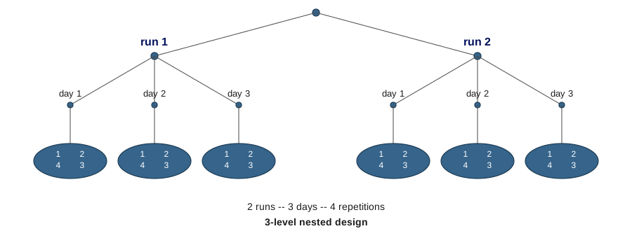
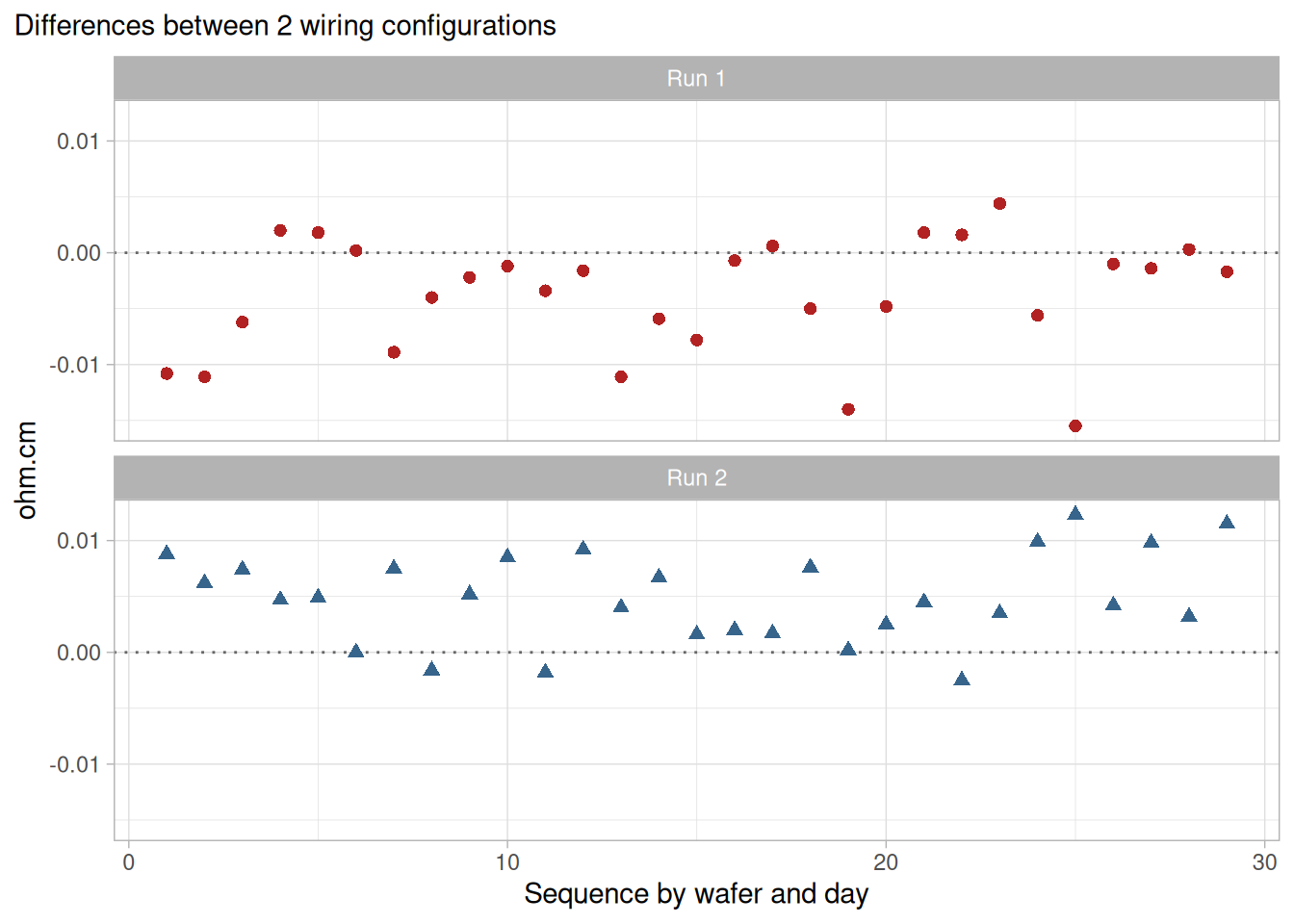
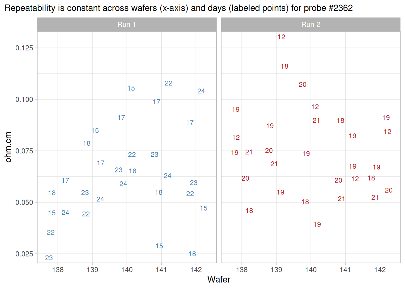
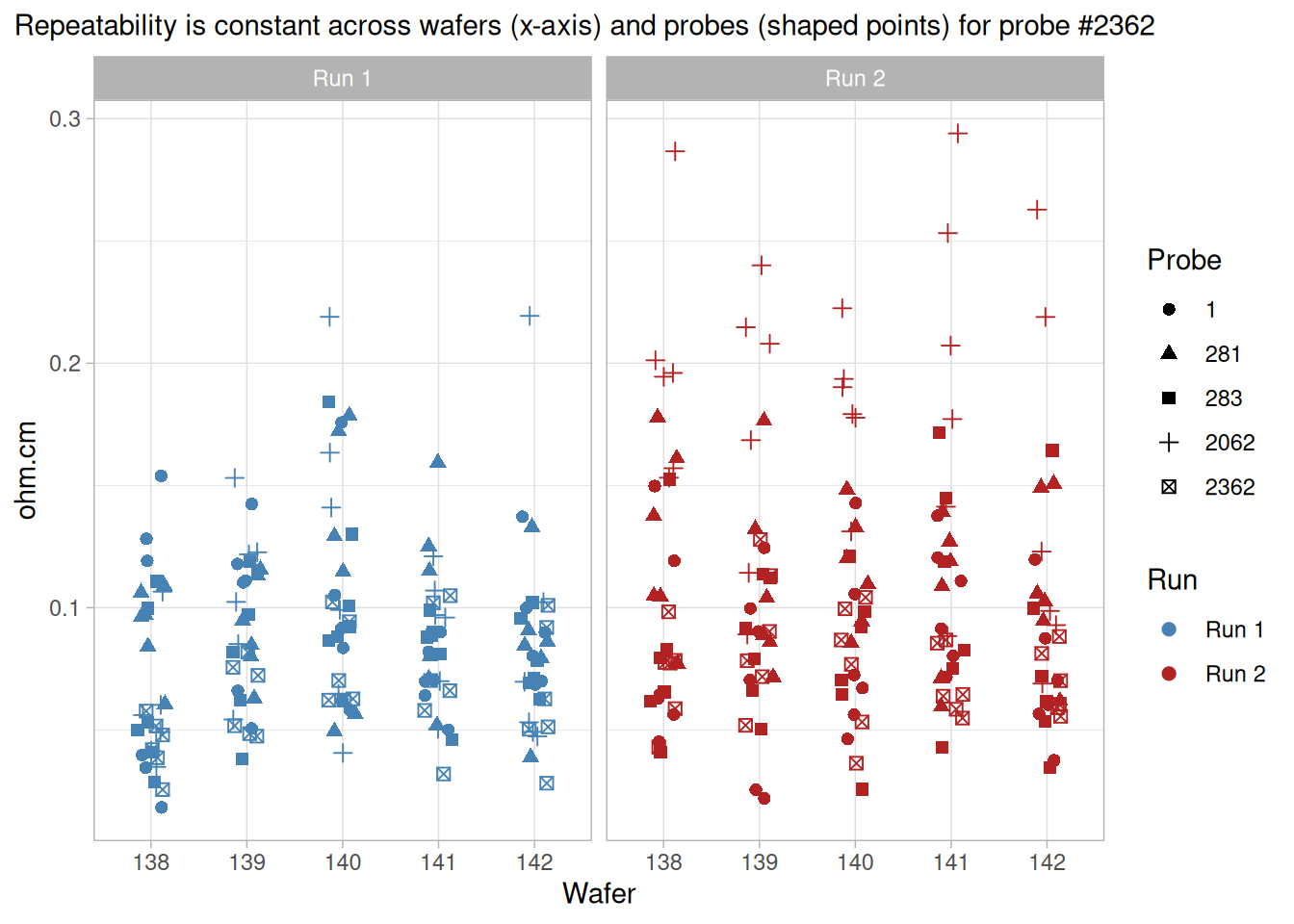
A measurement process can be thought of as a well-run production process in which measurements are the output. The ‘goodness’ of measurements is the issue, and goodness is characterized in terms of the errors that affect the measurements.
Bias, variability and uncertainty
The goodness of measurements is quantified in terms of
The continuation of goodness is guaranteed by a statistical control program that controls both
Short-term variability or instrument precision
Long-term variability which controls bias and day-to-day variability of the process
Scope is limited to ongoing processes
The techniques in this chapter are intended primarily for ongoing processes. One-time tests and special tests or destructive tests are difficult to characterize. Examples of ongoing processes are:
Calibration where similar test items are measured on a regular basis
Certification where materials are characterized on a regular basis
Production where the metrology (tool) errors may be significant
Special studies where data can be collected over the life of the study
Application to production processes
The material in this chapter is pertinent to the study of production processes for which the size of the metrology (tool) error may be an important consideration. More specific guidance on assessing metrology errors can be found in the section on gauge studies.
2.1.1.1 Purpose
Purpose is to understand and quantify the effect of error on reported values
The purpose of characterization is to develop an understanding of the sources of error in the measurement process and how they affect specific measurement results. This section provides the background for:
identifying sources of error in the measurement process
understanding and quantifying errors in the measurement process
codifying the effects of these errors on a specific reported value in a statement of uncertainty
Important concepts
Characterization relies upon the understanding of certain underlying concepts of measurement systems; namely,
Reported value is a generic term that identifies the result that is transmitted to the customer
The reported value is the measurement result for a particular test item. It can be:
a single measurement
an average of several measurements
a least-squares prediction from a model
a combination of several measurement results that are related by a physical model
2.1.1.2 Reference base
Ultimate authority
The most critical element of any measurement process is the relationship between a single measurement and the reference base for the unit of measurement. The reference base is the ultimate source of authority for the measurement unit.
For fundamental units
Reference bases for fundamental units of measurement (length, mass, temperature, voltage, and time) and some derived units (such as pressure, force, flow rate, etc.) are maintained by national and regional standards laboratories. Consensus values from interlaboratory tests or instrumentation/standards as maintained in specific environments may serve as reference bases for other units of measurement.
For comparison purposes
A reference base, for comparison purposes, may be based on an agreement among participating laboratories or organizations and derived from
measurements made with a standard test method
measurements derived from an interlaboratory test
2.1.1.3 Bias and Accuracy
Definition of Accuracy and Bias
Accuracy is a qualitative term referring to whether there is agreement between a measurement made on an object and its true (target or reference) value. Bias is a quantitative term describing the difference between the average of measurements made on the same object and its true value. In particular, for a measurement laboratory, bias is the difference (generally unknown) between a laboratory’s average value (over time) for a test item and the average that would be achieved by the reference laboratory if it undertook the same measurements on the same test item.
Depiction of bias and unbiased measurements
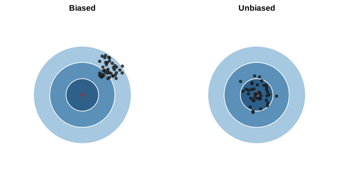
The traditional “dartboard” metaphor: unbiased measurements scatter around the bullseye (the target/true value), while biased measurements scatter around a point displaced from the bullseye.
Figure 2.1: Dartboard depiction of unbiased (left) and biased (right) measurements relative to a target
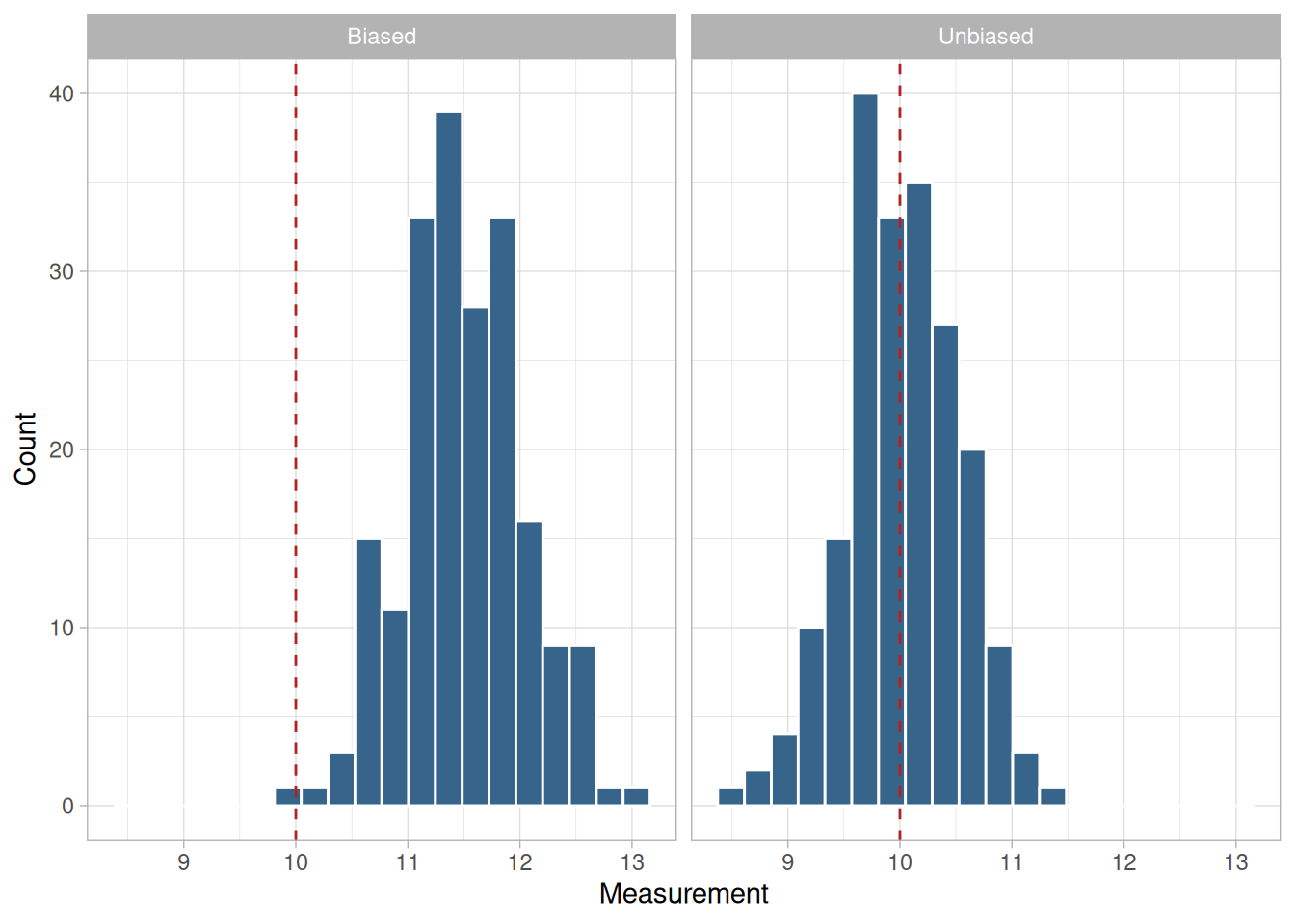
The same idea is shown below as a histogram of simulated measurements against the target value.
Code
library(tidyverse)set.seed(20240613)n_mpc113 <-200target_mpc113 <-10bias_demo_mpc113 <-bind_rows(tibble(y =rnorm(n_mpc113, mean = target_mpc113, sd =0.5), process ="Unbiased"),tibble(y =rnorm(n_mpc113, mean = target_mpc113 +1.5, sd =0.5), process ="Biased"))ggplot(bias_demo_mpc113, aes(y)) +geom_histogram(bins =20, color ="white", fill ="steelblue4") +geom_vline(xintercept = target_mpc113, color ="firebrick", linetype ="dashed") +facet_wrap(~process) +labs(x ="Measurement", y ="Count") +theme_light()
Figure 2.2: Simulated measurements relative to a target value, illustrating unbiased (left) and biased (right) measurement processes
The dashed line marks the target (true) value. Unbiased measurements are centered on the target; biased measurements are centered away from the target.
Identification of bias
Bias in a measurement process can be identified by:
Calibration of standards and/or instruments by a reference laboratory, where a value is assigned to the client’s standard based on comparisons with the reference laboratory’s standards.
Check standards, where violations of the control limits on a control chart for the check standard suggest that re-calibration of standards or instruments is needed.
Measurement assurance programs, where artifacts from a reference laboratory or other qualified agency are sent to a client and measured in the client’s environment as a ‘blind’ sample.
Interlaboratory comparisons, where reference standards or materials are circulated among several laboratories.
Reduction of bias
Bias can be eliminated or reduced by calibration of standards and/or instruments. Because of costs and time constraints, the majority of calibrations are performed by secondary or tertiary laboratories and are related to the reference base via a chain of intercomparisons that start at the reference laboratory.
Bias can also be reduced by corrections to in-house measurements based on comparisons with artifacts or instruments circulated for that purpose (reference materials).
Caution
Errors that contribute to bias can be present even where all equipment and standards are properly calibrated and under control. Temperature probably has the most potential for introducing this type of bias into the measurements. For example, a constant heat source will introduce serious errors in dimensional measurements of metal objects. Temperature affects chemical and electrical measurements as well.
Generally speaking, errors of this type can be identified only by those who are thoroughly familiar with the measurement technology. The reader is advised to consult the technical literature and experts in the field for guidance.
2.1.1.4 Variability
Sources of time-dependent variability
Variability is the tendency of the measurement process to produce slightly different measurements on the same test item, where conditions of measurement are either stable or vary over time, temperature, operators, etc. In this chapter we consider two sources of time-dependent variability:
Short-term variability ascribed to the precision of the instrument
Long-term variability related to changes in environment and handling techniques
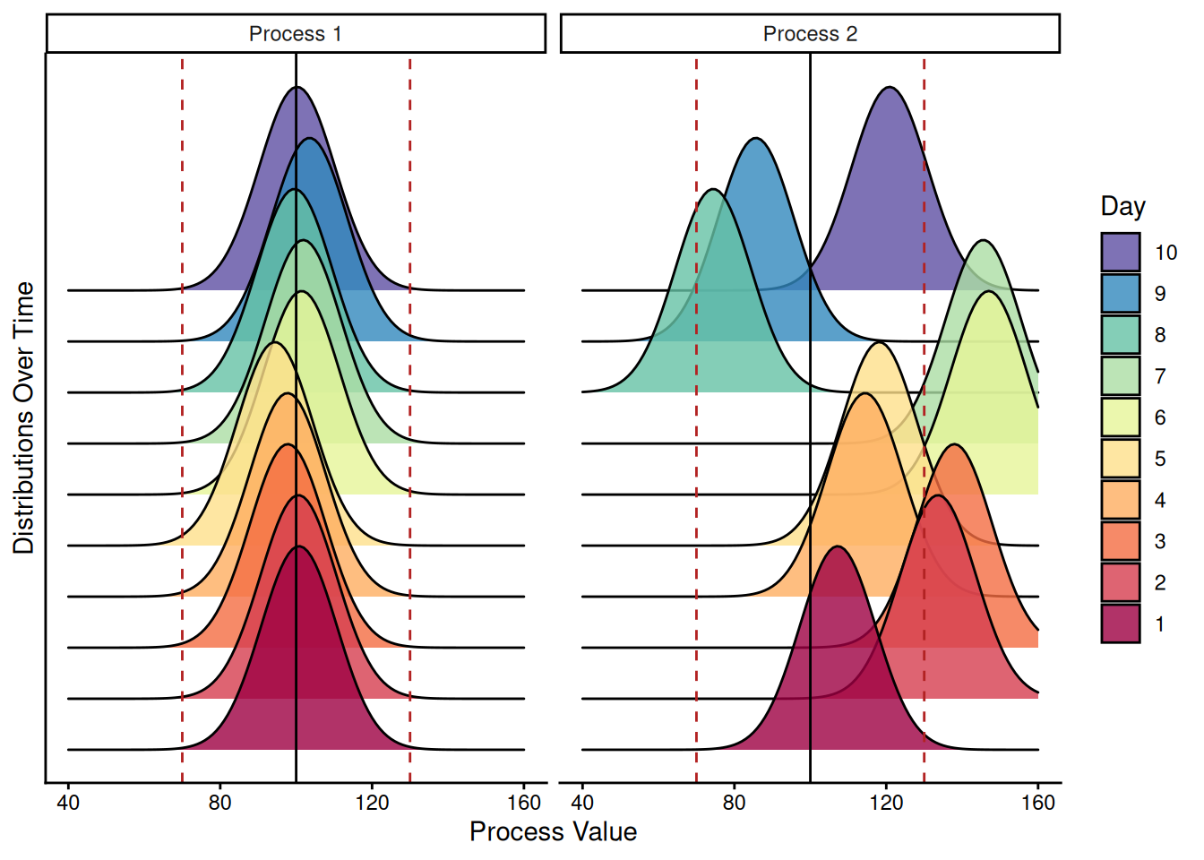
Depiction of two measurement processes with the same short-term variability over 10 days where process 1 has negligible between-day variability and process 2 has large between-day variability
Code
library(ggridges)set.seed(2020)label_mpc114 <-as_labeller(c(process_1 ="Process 1", process_2 ="Process 2"))dnorm_curve_mpc114 <-function(x) {dnorm(seq(40, 160, 1), mean = x, sd =10)}n_days_mpc114 <-10process_simulation_mpc114 <-tibble(day =seq_len(n_days_mpc114),process_1 =rnorm(n_days_mpc114, mean =100, sd =2),process_2 =rnorm(n_days_mpc114, mean =120, sd =15)) |>pivot_longer(c(process_1, process_2), names_to ="mean_process", values_to ="mean_values") |>mutate(simulated_distribution =map(mean_values, dnorm_curve_mpc114)) |>unnest(cols =c(simulated_distribution)) |>mutate(x_values =rep(seq(40, 160, 1), times =2* n_days_mpc114))process_simulation_mpc114 |>ggplot(aes(x = x_values, y = day, height = simulated_distribution *100, fill =as.factor(day))) +facet_wrap(vars(mean_process), labeller = label_mpc114) +geom_ridgeline(alpha =0.8) +geom_vline(xintercept =100, color ="black") +geom_vline(xintercept =c(70, 130), color ="firebrick", linetype ="dashed") +labs(x ="Process Value", y ="Distributions Over Time", fill ="Day") +guides(fill =guide_legend(reverse =TRUE)) +scale_fill_brewer(palette ="Spectral") +theme_classic() +theme(axis.text.y =element_blank(), axis.ticks.y =element_blank())
Figure 2.3: Simulated short-term measurement distributions over 10 days, illustrating small (process 1) versus large (process 2) between-day variability
Distributions of short-term measurements over 10 days where distances from the centerlines illustrate between-day variability.
Short-term variability
Short-term errors affect the precision of the instrument. Even very precise instruments exhibit small changes caused by random errors. It is useful to think in terms of measurements performed with a single instrument over minutes or hours; this is to be understood, normally, as the time that it takes to complete a measurement sequence.
Terminology
Four terms are in common usage to describe short-term phenomena. They are interchangeable.
precision
repeatability
within-time variability
short-term variability
Precision is quantified by a standard deviation
The measure of precision is a standard deviation. Good precision implies a small standard deviation. This standard deviation is called the short-term standard deviation of the process or the repeatability standard deviation.
Caution – long-term variability may be dominant
With very precise instrumentation, it is not unusual to find that the variability exhibited by the measurement process from day-to-day often exceeds the precision of the instrument because of small changes in environmental conditions and handling techniques which cannot be controlled or corrected in the measurement process. The measurement process is not completely characterized until this source of variability is quantified.
Terminology
Three terms are in common usage to describe long-term phenomena. They are interchangeable.
day-to-day variability
long-term variability
reproducibility
Caution – regarding term ‘reproducibility’
The term ‘reproducibility’ is given very specific definitions in some national and international standards. However, the definitions are not always in agreement. Therefore, it is used here only in a generic sense to indicate variability across days.
Definitions in this Handbook
We adopt precise definitions and provide data collection and analysis techniques in the sections on check standards and measurement control for estimating:
In the section on gauge studies, the concept of variability is extended to include very long-term measurement variability:
Level-1 standard deviation for short-term variability
Level-2 standard deviation for day-to-day variability
Level-3 standard deviation for very long-term variability
We refer to the standard deviations associated with these three kinds of uncertainty as “Level 1, 2, and 3 standard deviations”, respectively.
Long-term variability is quantified by a standard deviation
The measure of long-term variability is the standard deviation of measurements taken over several days, weeks or months.
The simplest method for doing this assessment is by analysis of a check standard database. The measurements on the check standards are structured to cover a long time interval and to capture all sources of variation in the measurement process.
2.1.2 What is a check standard?
A check standard is useful for gathering data on the process
Check standard methodology is a tool for collecting data on the measurement process to expose errors that afflict the process over time. Time-dependent sources of error are evaluated and quantified from the database of check standard measurements. It is a device for controlling the bias and long-term variability of the process once a baseline for these quantities has been established from historical data on the check standard.
Think in terms of data; a check standard can be an artifact or defined quantity
The check standard should be thought of in terms of a database of measurements. It can be defined as an artifact or as a characteristic of the measurement process whose value can be replicated from measurements taken over the life of the process. Examples are:
measurements on a stable artifact
differences between values of two reference standards as estimated from a calibration experiment
values of a process characteristic, such as a bias term, which is estimated from measurements on reference standards and/or test items.
An artifact check standard must be close in material content and geometry to the test items that are measured in the workload. If possible, it should be one of the test items from the workload. Obviously, it should be a stable artifact and should be available to the measurement process at all times.
Solves the difficulty of sampling the process
Measurement processes are similar to production processes in that they are continual and are expected to produce identical results (within acceptable limits) over time, instruments, operators, and environmental conditions. However, it is difficult to sample the output of the measurement process because, normally, test items change with each measurement sequence.
Surrogate for unseen measurements
Measurements on the check standard, spaced over time at regular intervals, act as surrogates for measurements that could be made on test items if sufficient time and resources were available.
2.1.2.1 Assumptions
Case study: Resistivity check standard
Before applying the quality control procedures recommended in this chapter to check standard data, basic assumptions should be examined. The basic assumptions underlying the quality control procedures are:
The data come from a single statistical distribution.
The distribution is a normal distribution.
The errors are uncorrelated over time.
An easy method for checking the assumption of a single normal distribution is to construct a histogram of the check standard data. The histogram should follow a bell-shaped pattern with a single hump. Types of anomalies that indicate a problem with the measurement system are:
a double hump indicating that errors are being drawn from two or more distributions;
long tails indicating outliers in the process;
flat pattern or one with humps at either end indicating that the measurement process in not in control or not properly specified.
Another graphical method for testing the normality assumption is a probability plot. The points are expected to fall approximately on a straight line if the data come from a normal distribution. Outliers, or data from other distributions, will produce an S-shaped curve.
A graphical method for testing for correlation among measurements is a time-lag plot. Correlation will frequently not be a problem if measurements are properly structured over time. Correlation problems generally occur when measurements are taken so close together in time that the instrument cannot properly recover from one measurement to the next. Correlations over time are usually present but are often negligible.
2.1.2.2 Data collection
Schedule for making measurements
A schedule for making check standard measurements over time (once a day, twice a week, or whatever is appropriate for sampling all conditions of measurement) should be set up and adhered to. The check standard measurements should be structured in the same way as values reported on the test items. For example, if the reported values are averages of two repetitions made within 5 minutes of each other, the check standard values should be averages of the two measurements made in the same manner.
Exception
One exception to this rule is that there should be at least \(J = 2\) repetitions per day. Without this redundancy, there is no way to check on the short-term precision of the measurement system.
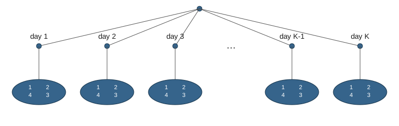
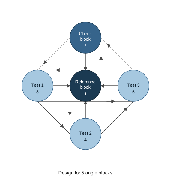
Depiction of schedule for making check standard measurements with four repetitions per day over K days on the surface of a silicon wafer with the repetitions at fixed positions on the wafer
Figure 2.4: A 2-level design for check standard measurements: J = 4 repetitions per day (sites 1-4 on the wafer) over K days
K days – 4 repetitions
Case study: Resistivity check standard for measurements on silicon wafers
The values for the check standard should be recorded along with pertinent environmental readings and identifications for all other significant factors. The best way to record this information is in one file with one line or row (on a spreadsheet) of information in fixed fields for each check standard measurement. A list of typical entries follows.
Identification for check standard
Date
Identification for the measurement design (if applicable)
Identification for the instrument
Check standard value
Short-term standard deviation from \(J\) repetitions
Degrees of freedom
Operator identification
Environmental readings (if pertinent)
2.1.2.3 Analysis
Short-term or level-1 standard deviations from J repetitions
An analysis of the check standard data is the basis for quantifying random errors in the measurement process – particularly time-dependent errors.
Given that we have a database of check standard measurements as described in data collection where
\[Y_{kj}\ (k=1, \ldots, K,\ j=1, \ldots, J)\]
represents the \(j\)th repetition on the \(k\)th day, the mean for the \(k\)th day is
An individual short-term standard deviation will not be a reliable estimate of precision if the degrees of freedom is less than ten, but the individual estimates can be pooled over the \(K\) days to obtain a more reliable estimate. The pooled level-1 standard deviation estimate with \(v = K(J - 1)\) degrees of freedom is
\[s_1 = \sqrt{\frac{1}{K} \sum_{k=1}^{K} s_k^2}\]
This standard deviation can be interpreted as quantifying the basic precision of the instrumentation used in the measurement process.
Process (level-2) standard deviation
The level-2 standard deviation of the check standard is appropriate for representing the process variability. It is computed with \(v = K - 1\) degrees of freedom as:
is the grand mean of the \(KJ\) check standard measurements.
Use in quality control
The check standard data and standard deviations that are described in this section are used for controlling two aspects of a measurement process:
Control of short-term variability
Control of bias and long-term variability
Case study: Resistivity check standard
For an example, see the case study for resistivity where several check standards were measured \(J = 6\) times per day over several days.
2.2 Statistical Control of a Measurement Process
The purpose of this section is to outline the steps that can be taken to exercise statistical control over the measurement process and demonstrate the validity of the uncertainty statement. Measurement processes can change both with respect to bias and variability. A change in instrument precision may be readily noted as measurements are being recorded, but changes in bias or long-term variability are difficult to catch when the process is looking at a multitude of artifacts over time.
2.2.1 What are the issues in controlling the measurement process?
Purpose is to guarantee the ‘goodness’ of measurement results
The purpose of statistical control is to guarantee the ‘goodness’ of measurement results within predictable limits and to validate the statement of uncertainty of the measurement result.
Statistical control methods can be used to test the measurement process for change with respect to bias and variability from its historical levels. However, if the measurement process is improperly specified or calibrated, then the control procedures can only guarantee comparability among measurements.
Assumption of normality is not stringent
The assumptions that relate to measurement processes apply to statistical control; namely that the errors of measurement are uncorrelated over time and come from a population with a single distribution. The tests for control depend on the assumption that the underlying distribution is normal (Gaussian), but the test procedures are robust to slight departures from normality. Practically speaking, all that is required is that the distribution of measurements be bell-shaped and symmetric.
Check standard is mechanism for controlling the process
Measurements on a check standard provide the mechanism for controlling the measurement process.
Measurements on the check standard should produce identical results except for the effect of random errors, and tests for control are basically tests of whether or not the random errors from the process continue to be drawn from the same statistical distribution as the historical data on the check standard.
Changes that can be monitored and tested with the check standard database are:
Bias and variability are controlled by monitoring measurements on a check standard over time
Bias and long-term variability are controlled by monitoring measurements on a check standard over time. A change in the measurement on the check standard that persists at a constant level over several measurement sequences indicates possible:
Change or damage to the reference standards
Change or damage to the check standard artifact
Procedural change that vitiates the assumptions of the measurement process
A change in the variability of the measurements on the check standard can be due to one of many causes such as:
Loss of environmental controls
Change in handling techniques
Severe degradation in instrumentation
The control procedure monitors the progress of measurements on the check standard over time and signals when a significant change occurs. There are two control chart procedures that are suitable for this purpose.
Shewhart Chart is easy to implement
The Shewhart control chart has the advantage of being intuitive and easy to implement. It is characterized by a center line and symmetric upper and lower control limits. The chart is good for detecting large changes but not for quickly detecting small changes (of the order of one-half to one standard deviation) in the process.
Depiction of Shewhart control chart
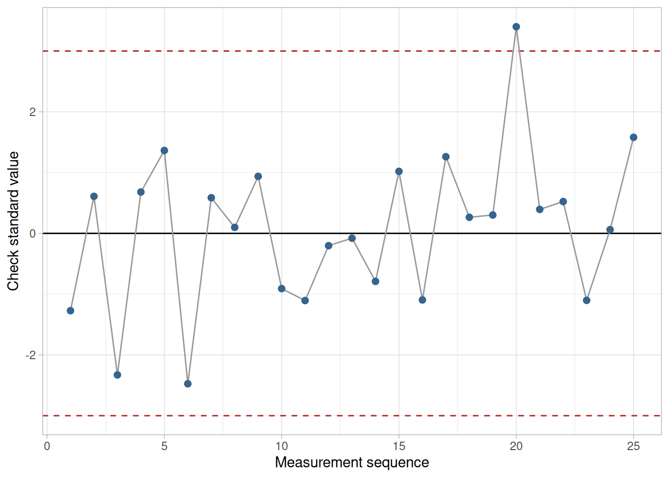
In the simplistic illustration of a Shewhart control chart shown below, the measurements are within the control limits with the exception of one measurement which exceeds the upper control limit.
Figure 2.5: Illustrative Shewhart control chart for a check standard: measurements are within the control limits except for one point that exceeds the upper control limit
EWMA Chart is better for detecting small changes
The EWMA control chart (exponentially weighted moving average) is more difficult to implement but should be considered if the goal is quick detection of small changes. The decision process for the EWMA chart is based on an exponentially decreasing (over time) function of prior measurements on the check standard while the decision process for the Shewhart chart is based on the current measurement only.
Example of EWMA Chart
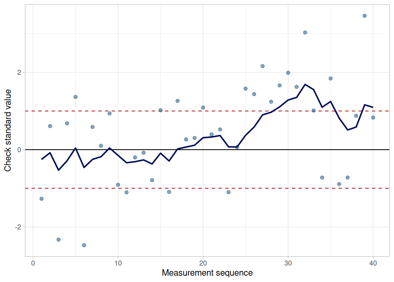
In the EWMA control chart below, the points represent the measurements (NIST’s original figure shows red dots; ours uses steelblue to match the book’s palette). Control is exercised via the exponentially weighted moving average (shown as the curved line) which, in this case, is approaching its upper control limit.
Figure 2.6: Illustrative EWMA control chart: the EWMA statistic (line) tracks a gradual drift in the raw check standard measurements (points) and approaches the upper control limit
Artifacts for process control must be stable and available
The check standard artifacts for controlling the bias or long-term variability of the process must be of the same type and geometry as items that are measured in the workload. The artifacts must be stable and available to the measurement process on a continuing basis. Usually, one artifact is sufficient. It can be:
An individual item drawn at random from the workload
A specific item reserved by the laboratory for the purpose
Example of Shewhart control chart for mass calibrations
The Shewhart control chart has a baseline and upper and lower limits, shown as dashed lines, that are symmetric about the baseline. Measurements are plotted on the chart versus a time line. Measurements that are outside the limits are considered to be out of control.
Baseline is the average from historical data
The baseline for the control chart is the accepted value, an average of the historical check standard values. A minimum of 100 check standard values is required to establish an accepted value.
Caution – control limits are computed from the process standard deviation – not from rational subsets
The upper (\(UCL\)) and lower (\(LCL\)) control limits are:
\[UCL = \text{Accepted value} + k \cdot \text{process standard deviation}\]\[LCL = \text{Accepted value} - k \cdot \text{process standard deviation}\]
where the process standard deviation is the standard deviation computed from the check standard database.
Individual measurements cannot be assessed using the standard deviation from short-term repetitions
This procedure is an individual observations control chart. The previously described control charts depended on rational subsets, which use the standard deviations computed from the rational subsets to calculate the control limits. For a measurement process, the subgroups would consist of short-term repetitions which can characterize the precision of the instrument but not the long-term variability of the process. In measurement science, the interest is in assessing individual measurements (or averages of short-term repetitions). Thus, the standard deviation over time is the appropriate measure of variability.
Choice of k depends on number of measurements we are willing to reject
To achieve tight control of the measurement process, set \(k = 2\), in which case approximately 5% of the measurements from a process that is in control will produce out-of-control signals. This assumes that there is a sufficiently large number of degrees of freedom (\(>100\)) for estimating the process standard deviation.
To flag only those measurements that are egregiously out of control, set \(k = 3\), in which case approximately 1% of the measurements from an in-control process will produce out-of-control signals.
See Figure 2.5 above for a depiction of a Shewhart control chart.
2.2.2.2 EWMA control chart
Small changes only become obvious over time
Because it takes time for the patterns in the data to emerge, a permanent shift in the process may not immediately cause individual violations of the control limits on a Shewhart control chart. The Shewhart control chart is not powerful for detecting small changes, say of the order of 1-1/2 standard deviations. The EWMA (exponentially weighted moving average) control chart is better suited to this purpose.
Example of EWMA control chart for mass calibrations
The exponentially weighted moving average (EWMA) is a statistic for monitoring the process that averages the data in a way that gives less and less weight to data as they are further removed in time from the current measurement. The data \(Y_1, Y_2, \ldots, Y_t\) are the check standard measurements ordered in time. The EWMA statistic at time \(t\) is computed recursively from individual data points, with the first EWMA statistic, \(EWMA_1\), being the arithmetic average of historical data.
\[EWMA_{t+1} = \lambda Y_t + (1-\lambda) EWMA_t\]
Control mechanism for EWMA
The EWMA control chart can be made sensitive to small changes or a gradual drift in the process by the choice of the weighting factor, \(\lambda\). A weighting factor of 0.2-0.3 is usually suggested for this purpose (Hunter 1986), and 0.15 is also a popular choice.
Limits for the control chart
The target or center line for the control chart is the average of historical data. The upper (\(UCL\)) and lower (\(LCL\)) limits are
where \(s\) times the radical expression is a good approximation to the standard deviation of the EWMA statistic and the factor \(k\) is chosen in the same way as for the Shewhart control chart – generally to be 2 or 3.
Procedure for implementing the EWMA control chart
The implementation of the EWMA control chart is the same as for any other type of control procedure. The procedure is built on the assumption that the “good” historical data are representative of the in-control process, with future data from the same process tested for agreement with the historical data. To start the procedure, a target (average) and process standard deviation are computed from historical check standard data. Then the procedure enters the monitoring stage with the EWMA statistics computed and tested against the control limits. The EWMA statistics are weighted averages, and thus their standard deviations are smaller than the standard deviations of the raw data and the corresponding control limits are narrower than the control limits for the Shewhart individual observations chart.
See Figure 2.6 above for a depiction of an EWMA control chart.
2.2.2.3 Data collection
Measurements should cover a sufficiently long time period to cover all environmental conditions
A schedule should be set up for making measurements on the artifact (check standard) chosen for control purposes. The measurements are structured to sample all environmental conditions in the laboratory and all other sources of influence on the measurement result, such as operators and instruments.
For high-precision processes where the uncertainty of the result must be guaranteed, a measurement on the check standard should be included with every measurement sequence, if possible, and at least once a day.
For each occasion, \(J\) measurements are made on the check standard. If there is no interest in controlling the short-term variability or precision of the instrument, then one measurement is sufficient. However, a dual purpose is served by making two or three measurements that track both the bias and the short-term variability of the process with the same database.
Depiction of check standard measurements
Depiction of check standard measurements with J = 4 repetitions per day on the surface of a silicon wafer over K days where the repetitions are at fixed positions on the wafer (see Figure 2.4).
Notation
For \(J\) measurements on each of \(K\) days, the measurements are denoted by
\[Y_{kj}\ (k=1,\ldots,K,\ j=1,\ldots,J)\]
The check standard value is defined as an average of short-term repetitions
Check standard measurements should be structured in the same way as values reported on the test items. For example, if the reported values are averages of two measurements made within 5 minutes of each other, the check standard values should be averages of the two measurements made in the same manner.
Database
Averages and short-term standard deviations computed from \(J\) repetitions should be recorded in a file along with identifications for all significant factors. The best way to record this information is to use one file with one line (row in a spreadsheet) of information in fixed fields for each group. A list of typical entries follows:
Month
Day
Year
Check standard identification
Identification for the measurement design (if applicable)
Instrument identification
Check standard value
Repeatability (short-term) standard deviation from \(J\) repetitions
Degrees of freedom
Operator identification
Environmental readings (if pertinent)
Case Study
Check standard for resistivity measurements
2.2.2.4 Monitoring bias and long-term variability
Monitoring stage
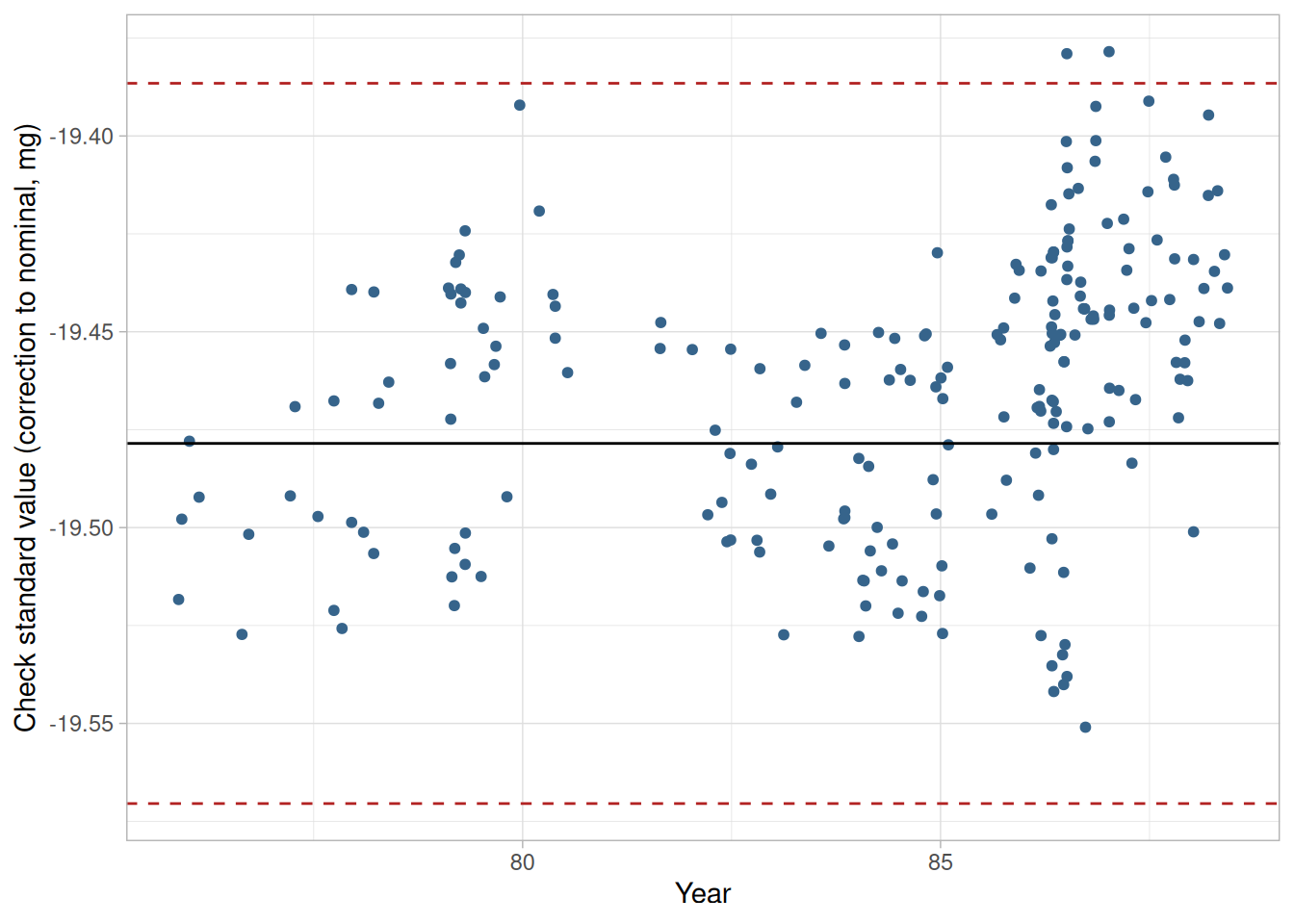
Once the baseline and control limits for the control chart have been determined from historical data, and any bad observations removed and the control limits recomputed, the measurement process enters the monitoring stage. A Shewhart control chart and EWMA control chart for monitoring a mass calibration process are shown below. For the purpose of comparing the two techniques, the two control charts are based on the same data where the baseline and control limits are computed from the data taken prior to 1985. The monitoring stage begins at the start of 1985. Similarly, the control limits for both charts are 3-standard deviation limits. The check standard data and analysis are explained more fully in another section.
Shewhart control chart of measurements of kilogram check standard showing outliers and a shift in the process that occurred after 1985
Code
library(tidyverse)mass_mpc223 <-read_table( here::here("datasets", "MASS.DAT"),skip =25,col_names =c("date_year", "std_id", "std_value", "balance_id", "std_dev", "design_id"),col_types ="dddddd")mn_mpc223 <-mean(mass_mpc223$std_value[mass_mpc223$date_year <85])std_mpc223 <-sd(mass_mpc223$std_value[mass_mpc223$date_year <85])lcl_mpc223 <- mn_mpc223 -3* std_mpc223ucl_mpc223 <- mn_mpc223 +3* std_mpc223ggplot(mass_mpc223, aes(date_year, std_value)) +geom_point(color ="steelblue4", size =1.4) +geom_hline(yintercept = mn_mpc223, color ="black") +geom_hline(yintercept =c(lcl_mpc223, ucl_mpc223), color ="firebrick", linetype ="dashed") +labs(x ="Year", y ="Check standard value (correction to nominal, mg)") +theme_light()
Figure 2.7: Shewhart control chart of kilogram check standard measurements (1975-1988): baseline and 3-standard-deviation control limits computed from data prior to 1985
The control chart shows only two violations of the control limits before 1985. For those occasions, the calibrations were discarded and repeated. After 1985, the points cluster increasingly close to and above the upper control limit – an unequal distribution of data points on the two sides of the baseline that indicates a change in either the process average (possibly related to a change in the reference standards) or the variability (possibly caused by a change in the instrument precision).
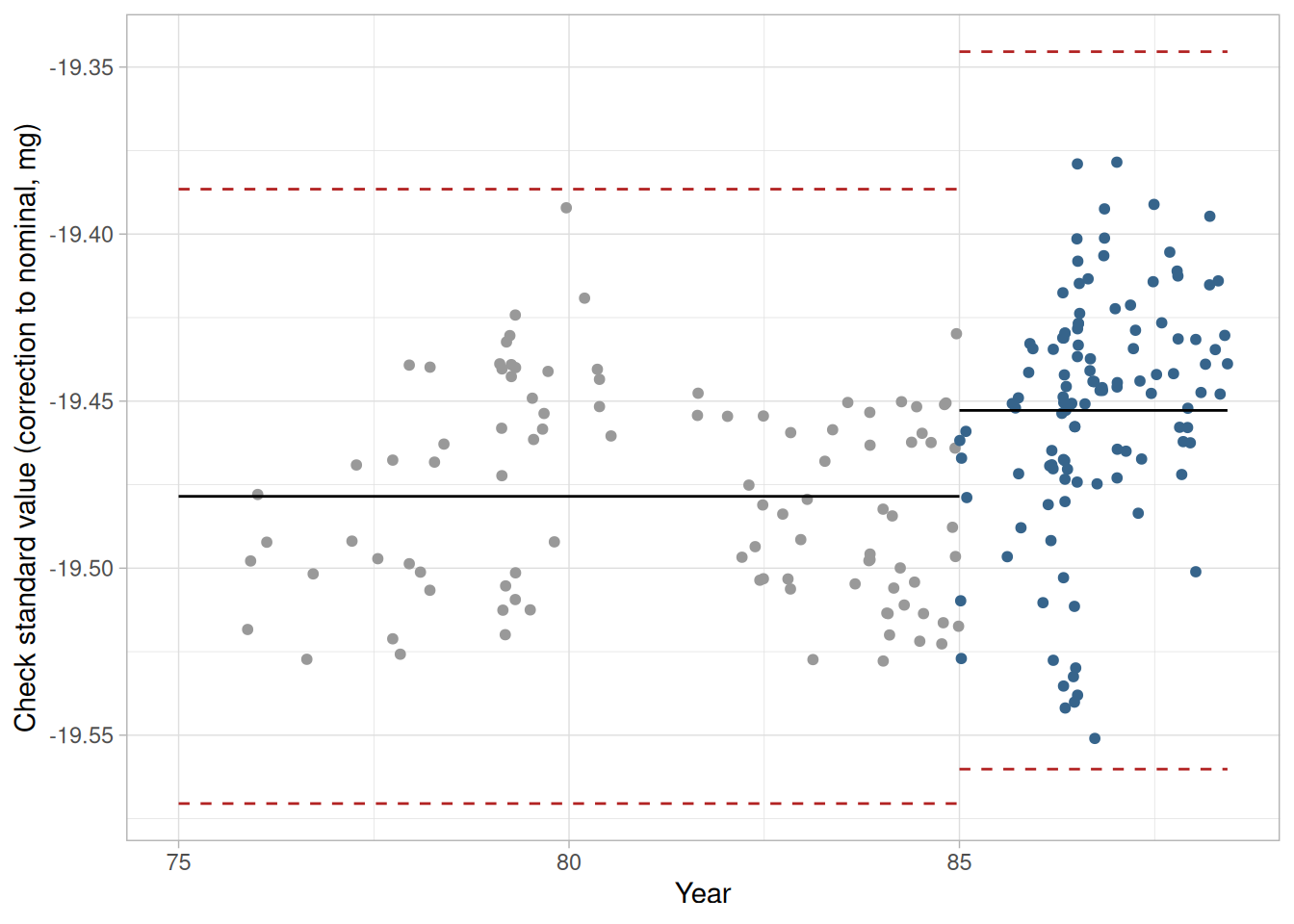
Unfortunately, it takes time for the patterns in the data to emerge because individual violations of the control limits do not necessarily point to a permanent shift in the process. If the limits for the control chart are re-calculated based on the data after 1985, the extent of the change is obvious.
Revised control chart based on check standard measurements after 1985
Figure 2.8: Revised Shewhart control chart for kilogram check standard measurements: baseline and control limits computed separately for data prior to 1985 and data after 1985
Because the exponentially weighted moving average (EWMA) control chart is capable of detecting small changes, it may be a better choice for a high precision process that is producing many control values.
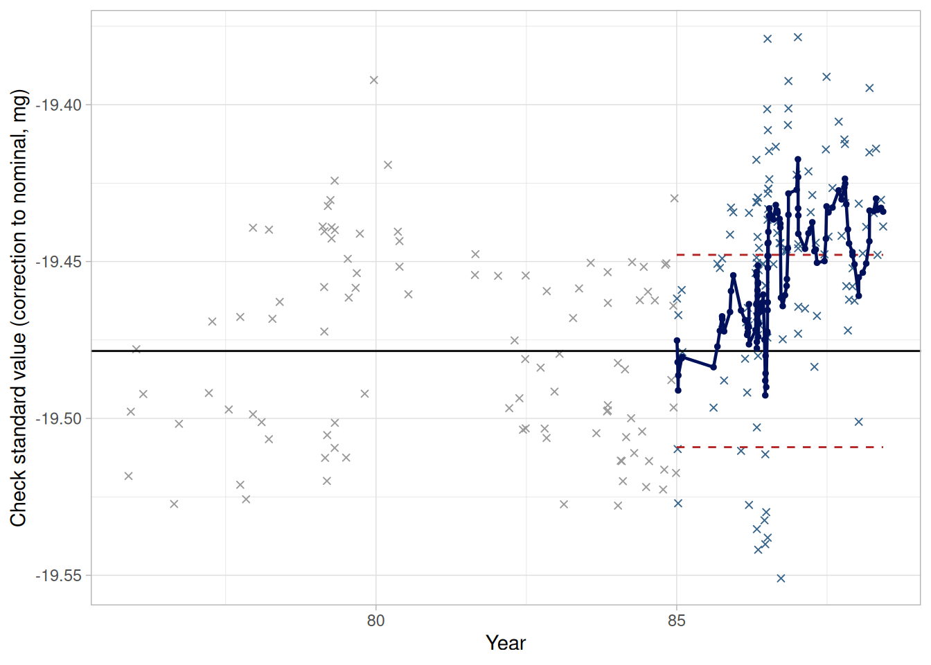
EWMA chart for measurements on kilogram check standard showing multiple violations of the control limits for the EWMA statistics
Code
library(tidyverse)lambda_mpc223 <-0.2k_mpc223 <-3ucl_ewma_mpc223 <- mn_mpc223 + std_mpc223 * k_mpc223 *sqrt(lambda_mpc223 / (2- lambda_mpc223))lcl_ewma_mpc223 <- mn_mpc223 - std_mpc223 * k_mpc223 *sqrt(lambda_mpc223 / (2- lambda_mpc223))ind_mpc223 <-which(mass_mpc223$date_year >85)ewma_mpc223 <-numeric(length(ind_mpc223) +1)ewma_mpc223[1] <- mn_mpc223for (i inseq_along(ind_mpc223)) { ewma_mpc223[i +1] <- lambda_mpc223 * mass_mpc223$std_value[ind_mpc223[i]] + (1- lambda_mpc223) * ewma_mpc223[i]}ewma_tbl_mpc223 <-tibble(date_year = mass_mpc223$date_year[ind_mpc223], ewma = ewma_mpc223[-1])ggplot(mass_mpc223, aes(date_year, std_value)) +geom_point(aes(color = date_year >85), size =1.4, shape =4) +scale_color_manual(values =c("grey60", "steelblue4"), guide ="none") +geom_hline(yintercept = mn_mpc223, color ="black") +annotate("segment", x =85, xend =max(mass_mpc223$date_year), y = ucl_ewma_mpc223, yend = ucl_ewma_mpc223, color ="firebrick", linetype ="dashed") +annotate("segment", x =85, xend =max(mass_mpc223$date_year), y = lcl_ewma_mpc223, yend = lcl_ewma_mpc223, color ="firebrick", linetype ="dashed") +geom_line(data = ewma_tbl_mpc223, aes(date_year, ewma), color ="#00105A", linewidth =0.8) +geom_point(data = ewma_tbl_mpc223, aes(date_year, ewma), color ="#00105A", size =1) +labs(x ="Year", y ="Check standard value (correction to nominal, mg)") +theme_light()
Figure 2.9: EWMA control chart of kilogram check standard measurements: target and process standard deviation from data prior to 1985, lambda = 0.2, k = 3
The target (average) and process standard deviation are computed from the check standard data taken prior to 1985. The computation of the EWMA statistic begins with the data taken at the start of 1985. In the control chart above, the raw data after 1985 are shown in steelblue (NIST’s original figure uses green for the raw data after 1985, black dots for the EWMA statistic, and red for the control limits; we use steelblue for the post-1985 raw data and the book’s dark navy for the EWMA statistic to match our palette), and the EWMA statistics are shown as the dark navy line superimposed on the raw data. The control limits are calculated according to the equation above where the process standard deviation, \(s =\) 0.03065 mg and \(k = 3\). The EWMA statistics, and not the raw data, are of interest in looking for out-of-control signals. The EWMA control chart shows many violations of the control limits starting at approximately the mid-point of 1986. This pattern emerges because the process average has actually shifted about one standard deviation, and the EWMA control chart is sensitive to small changes.
Measurements that exceed the control limits require action
The control strategy is based on the predictability of future measurements from historical data. Each new check standard measurement is plotted on the control chart in real time. These values are expected to fall within the control limits if the process has not changed. Measurements that exceed the control limits are probably out-of-control and require remedial action. Possible causes of out-of-control signals need to be understood when developing strategies for dealing with outliers.
Signs of significant trends or shifts
The control chart should be viewed in its entirety on a regular basis to identify drift or shift in the process. In the Shewhart control chart shown above, only a few points exceed the control limits. The small, but significant, shift in the process that occurred after 1985 can only be identified by examining the plot of control measurements over time. A re-analysis of the kilogram check standard data shows that the control limits for the Shewhart control chart should be updated based on the data after 1985. In the EWMA control chart, multiple violations of the control limits occur after 1986. In the calibration environment, the incidence of several violations should alert the control engineer that a shift in the process has occurred, possibly because of damage or change in the value of a reference standard, and the process requires review.
2.2.2.5 Remedial actions
Consider possible causes for out-of-control signals and take corrective long-term actions
There are many possible causes of out-of-control signals.
A. Causes that do not warrant corrective action for the process (but which do require that the current measurement be discarded) are:
Chance failure where the process is actually in control
Glitch in setting up or operating the measurement process
Error in recording of data
B. Changes in bias can be due to:
Damage to artifacts
Degradation in artifacts (wear or build-up of dirt and mineral deposits)
C. Changes in long-term variability can be due to:
Degradation in the instrumentation
Changes in environmental conditions
Effect of a new or inexperienced operator
4-step strategy for short-term
An immediate strategy for dealing with out-of-control signals associated with high precision measurement processes should be pursued as follows:
Repeat measurements. Repeat the measurement sequence to establish whether or not the out-of-control signal was simply a chance occurrence, glitch, or whether it flagged a permanent change or trend in the process.
Discard measurements on test items. With high precision processes, for which a check standard is measured along with the test items, new values should be assigned to the test items based on new measurement data.
Check for drift. Examine the patterns of recent data. If the process is gradually drifting out of control because of degradation in instrumentation or artifacts, then instruments may need to be repaired, or reference artifacts may need to be recalibrated.
Reevaluate. Reestablish the process value and control limits from more recent data if the measurement process cannot be brought back into control.
2.2.3 How is short-term variability controlled?
Emphasis on instruments
Short-term variability or instrument precision is controlled by monitoring standard deviations from repeated measurements on the instrument(s) of interest. The database can come from measurements on a single artifact or a representative set of artifacts.
Artifacts – Case study: Resistivity
The artifacts must be of the same type and geometry as items that are measured in the workload, such as:
Items from the workload
A single check standard chosen for this purpose
A collection of artifacts set aside for this specific purpose
Degradation of instrument or anomalous behavior on one occasion
Changes in the precision of the instrument, particularly anomalies and degradation, must be addressed. Changes in precision can be detected by a statistical control procedure based on the \(F\)-distribution where the short-term standard deviations are plotted on the control chart.
The base line for this type of control chart is the pooled standard deviation, \(s_1\), as defined in Data collection and analysis.
Example of control chart for a mass balance
Only the upper control limit, \(UCL\), is of interest for detecting degradation in the instrument. As long as the short-term standard deviations fall within the upper control limit established from historical data, there is reason for confidence that the precision of the instrument has not degraded (i.e., common cause variations).
The control limit is based on the F-distribution
The control limit is
\[UCL = s_1 \sqrt{F_{\alpha,\ J-1,\ K(J-1)}}\]
where the quantity under the radical is the upper \(\alpha\) critical value from the F table with degrees of freedom \((J-1)\) and \(K(J-1)\). The numerator degrees of freedom, \(v_1 = (J-1)\), are associated with the standard deviation computed from the current measurements, and the denominator degrees of freedom, \(v_2 = K(J-1)\), correspond to the pooled standard deviation of the historical data. The probability \(\alpha\) is chosen to be small, say 0.05.
The justification for this control limit, as opposed to the more conventional standard deviation control limit, is that we are essentially performing the following hypothesis test:
where \(\sigma_1\) is the population value for the \(s_1\) defined above and \(\sigma_2\) is the value against which the standard deviation of the current value is being tested. Generally, \(s_1\) is based on sufficient historical data that it is reasonable to make the assumption that \(\sigma_1\) is a “known” value.
The upper control limit above is then derived based on the standard \(F\) test for equal standard deviations. Justification and details of this derivation are given in Cameron and Hailes (1974).
Sample Code
For \(\alpha = 0.05\), \(J = 6\), and \(K = 6\), the critical value and control limit are computed as follows.
The computed critical value is \(F_{0.05,\,5,\,30} \approx\) 2.5336, matching NIST’s own sample calculation for this case.
2.2.3.2 Data collection
Case Study
Check standard for resistivity measurements
A schedule should be set up for making measurements with a single instrument (once a day, twice a week, or whatever is appropriate for sampling all conditions of measurement).
Short-term standard deviations
The measurements are denoted
\[Y_{kj}\ (k=1,\ldots,K,\ j=1,\ldots,J)\]
where there are \(J\) measurements on each of \(K\) occasions. The average for the \(k\)th occasion is:
The repeatability standard deviations are pooled over the \(K\) occasions to obtain an estimate with \(K(J-1)\) degrees of freedom of the level-1 standard deviation
\[s_1 = \sqrt{\frac{1}{K}\sum_{k=1}^{K} s_k^2}\]
Note: The same notation is used for the repeatability standard deviation whether it is based on one set of measurements or pooled over several sets.
Database
The individual short-term standard deviations along with identifications for all significant factors are recorded in a file. The best way to record this information is by using one file with one line (row in a spreadsheet) of information in fixed fields for each group. A list of typical entries follows:
Identification of test item or check standard
Date
Short-term standard deviation
Degrees of freedom
Instrument
Operator
2.2.3.3 Monitoring short-term precision
Monitoring future precision
Once the base line and control limit for the control chart have been determined from historical data, the measurement process enters the monitoring stage. In the control chart shown below, the control limit is based on historical standard deviations pooled from the check standard data (NIST’s own sample code pools the full historical record from 1975-1988 rather than only data prior to 1985 as the surrounding narrative describes; we follow the sample code, since it is what reproduces NIST’s stated control limit of 0.067 micrograms).
Each new standard deviation is monitored on the control chart
Each new short-term standard deviation based on \(J\) measurements is plotted on the control chart; points that exceed the control limits probably indicate lack of statistical control. Drift over time indicates degradation of the instrument. Points out of control require remedial action, and possible causes of out-of-control signals need to be understood when developing strategies for dealing with outliers.
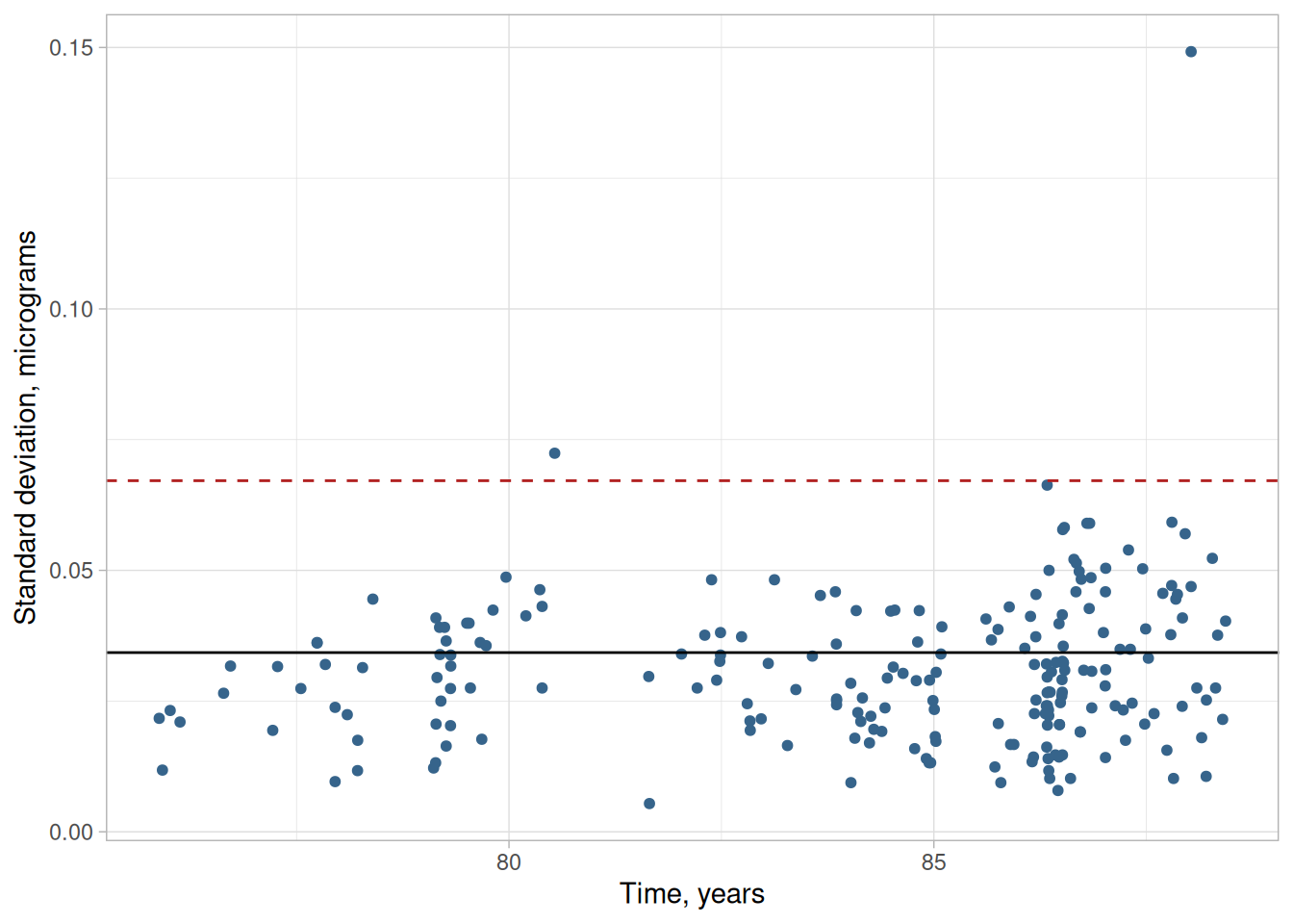
Control chart for precision for a mass balance from historical standard deviations for the balance with 3 degrees of freedom each. The control chart identifies two outliers and slight degradation over time in the precision of the balance
Figure 2.10: Control chart for precision of balance #12: standard deviations with 3 degrees of freedom plotted vs. year, with the upper control limit computed at the 1% significance level
The pooled standard deviation is \(s_1 \approx\) 0.03428 micrograms, and the control limit at the 1% significance level is 0.067 micrograms (dashed line), matching NIST’s stated control limit of 0.067 micrograms. The control chart shows that the precision of the balance remained in control through the first five months of 1988 with only two violations of the control limits. For those occasions, the calibrations were discarded and repeated. Clearly, for the second violation, something significant occurred that invalidated the calibration results. However, it is also clear from the pattern of standard deviations over time that the precision of the balance was gradually degrading and more and more points were approaching the control limits. This finding led to a decision to replace this balance for high accuracy calibrations.
Monitoring where the number of measurements are different from J
There is no requirement that future standard deviations be based on \(J\), the number of measurements in the historical database. However, a change in the number of measurements leads to a change in the test for control, and it may not be convenient to draw a control chart where the control limits are changing with each new measurement sequence.
For a new standard deviation based on \(J'\) measurements, the precision of the instrument is in control if
Notice that the numerator degrees of freedom, \(v_1 = J' - 1\), changes but the denominator degrees of freedom, \(v_2 = K(J-1)\), remains the same.
2.2.3.4 Remedial actions
Examine possible causes
A. Causes that do not warrant corrective action (but which do require that the current measurement be discarded) are:
Chance failure where the precision is actually in control
Glitch in setting up or operating the measurement process
Error in recording of data
B. Changes in instrument performance can be due to:
Degradation in electronics or mechanical components
Changes in environmental conditions
Effect of a new or inexperienced operator
Repeat measurements
Repeat the measurement sequence to establish whether or not the out-of-control signal was simply a chance occurrence, glitch, or whether it flagged a permanent change or trend in the process.
Assign new value to test item
With high precision processes, for which the uncertainty must be guaranteed, new values should be assigned to the test items based on new measurement data.
Check for degradation
Examine the patterns of recent standard deviations. If the process is gradually drifting out of control because of degradation in instrumentation or artifacts, instruments may need to be repaired or replaced.
2.3 Calibration
The purpose of this section is to outline the procedures for calibrating artifacts and instruments while guaranteeing the ‘goodness’ of the calibration results. Calibration is a measurement process that assigns values to the property of an artifact or to the response of an instrument relative to reference standards or to a designated measurement process. The purpose of calibration is to eliminate or reduce bias in the user’s measurement system relative to the reference base. The calibration procedure compares an “unknown” or test item(s) or instrument with reference standards according to a specific algorithm.
Calibration is a measurement process that assigns values to the property of an artifact or to the response of an instrument relative to reference standards or to a designated measurement process. The purpose of calibration is to eliminate or reduce bias in the user’s measurement system relative to the reference base.
Artifact & instrument calibration
The calibration procedure compares an “unknown” or test item(s) or instrument with reference standards according to a specific algorithm. Two general types of calibration are considered in this Handbook:
The procedures in this Handbook are appropriate for calibrations at secondary or lower levels of the traceability chain where reference standards for the unit already exist. Calibration from first principles of physics and reciprocity calibration are not discussed.
2.3.1.1 Reference base
Ultimate authority
The most critical element of any measurement process is the relationship between a single measurement and the reference base for the unit of measurement. The reference base is the ultimate source of authority for the measurement unit.
Base and derived units of measurement
The base units of measurement in the Le Systeme International d’Unites (SI) are (Taylor 1991):
kilogram - mass
meter - length
second - time
ampere - electric current
kelvin - thermodynamic temperature
mole - amount of substance
candela - luminous intensity
These units are maintained by the Bureau International des Poids et Mesures in Paris. Local reference bases for these units and SI derived units such as:
pascal - pressure
newton - force
hertz - frequency
ohm - resistance
degrees Celsius - Celsius temperature, etc.
are maintained by national and regional standards laboratories.
Other sources
Consensus values from interlaboratory tests or instrumentation/standards as maintained in specific environments may serve as reference bases for other units of measurement.
2.3.1.2 Reference standards
Primary reference standards
A reference standard for a unit of measurement is an artifact that embodies the quantity of interest in a way that ties its value to the reference base.
At the highest level, a primary reference standard is assigned a value by direct comparison with the reference base. Mass is the only unit of measurement that is defined by an artifact. The kilogram is defined as the mass of a platinum-iridium kilogram that is maintained by the Bureau International des Poids et Mesures in Sevres, France. (This reflects the SI definition in effect when NIST wrote this text; since the 2019 redefinition of the SI, the kilogram is instead defined by fixing the numerical value of the Planck constant, and the platinum-iridium artifact is no longer the primary reference.)
Primary reference standards for other units come from realizations of the units embodied in artifact standards. For example, the reference base for length is the meter which is defined as the length of the path by light in vacuum during a time interval of 1/299,792,458 of a second.
Secondary reference standards
Secondary reference standards are calibrated by comparing with primary standards using a high precision comparator and making appropriate corrections for non-ideal conditions of measurement.
Secondary reference standards for mass are stainless steel kilograms, which are calibrated by comparing with a primary standard on a high precision balance and correcting for the buoyancy of air. In turn these weights become the reference standards for assigning values to test weights.
Secondary reference standards for length are gage blocks, which are calibrated by comparing with primary gage block standards on a mechanical comparator and correcting for temperature. In turn, these gage blocks become the reference standards for assigning values to test sets of gage blocks.
2.3.2 What is artifact (single-point) calibration?
Purpose
Artifact calibration is a measurement process that assigns values to the property of an artifact relative to a reference standard(s). The purpose of calibration is to eliminate or reduce bias in the user’s measurement system relative to the reference base.
The calibration procedure compares an “unknown” or test item(s) with a reference standard(s) of the same nominal value (hence, the term single-point calibration) according to a specific algorithm called a calibration design.
Assumptions
The calibration procedure is based on the assumption that individual readings on test items and reference standards are subject to:
Bias that is a function of the measuring system or instrument
Random error that may be uncontrollable
What is bias?
The operational definition of bias is that it is the difference between values that would be assigned to an artifact by the client laboratory and the laboratory maintaining the reference standards. Values, in this sense, are understood to be the long-term averages that would be achieved in both laboratories.
Calibration model for eliminating bias requires a reference standard that is very close in value to the test item
One approach to eliminating bias is to select a reference standard that is almost identical to the test item; measure the two artifacts with a comparator type of instrument; and take the difference of the two measurements to cancel the bias. The only requirement on the instrument is that it be linear over the small range needed for the two artifacts.
The test item has value \(X^*\), as yet to be assigned, and the reference standard has an assigned value \(R^*\). Given a measurement, \(X\), on the test item and a measurement, \(R\), on the reference standard,
\[
\begin{aligned}
X &= Bias + X^* + error_1 \\
R &= Bias + R^* + error_2
\end{aligned}
\]
the difference between the test item and the reference is estimated by
\[D = X - R \, ,\]
and the value of the test item is reported as
\[\widehat{Test} = X^* = D + R^* \, .\]
Need for redundancy leads to calibration designs
A deficiency in relying on a single difference to estimate \(D\) is that there is no way of assessing the effect of random errors. The obvious solution is to:
Repeat the calibration measurements \(J\) times
Average the results
Compute a standard deviation from the \(J\) results
Schedules of redundant intercomparisons involving measurements on several reference standards and test items in a connected sequence are called calibration designs and are discussed in later sections.
2.3.3 What are calibration designs?
Calibration designs are redundant schemes for intercomparing reference standards and test items
Calibration designs are redundant schemes for intercomparing reference standards and test items in such a way that the values can be assigned to the test items based on known values of reference standards. Artifacts that traditionally have been calibrated using calibration designs are:
Assumptions for calibration designs include demands on the quality of the artifacts
The assumptions that are necessary for working with calibration designs are that:
Random errors associated with the measurements are independent.
All measurements come from a distribution with the same standard deviation.
Reference standards and test items respond to the measuring environment in the same manner.
Handling procedures are consistent from item to item.
Reference standards and test items are stable during the time of measurement.
Bias is canceled by taking the difference between measurements on the test item and the reference standard.
Important concept - Restraint
The restraint is the known value of the reference standard or, for designs with two or more reference standards, the restraint is the summation of the values of the reference standards.
Requirements & properties of designs
Basic requirements are:
The differences must be nominally zero.
The design must be solvable for individual items given the restraint.
It is possible to construct designs which do not have these properties. This will happen, for example, if reference standards are only compared among themselves and test items are only compared among themselves without any intercomparisons.
Practical considerations determine a ‘good’ design
We do not apply ‘optimality’ criteria in constructing calibration designs because the construction of a ‘good’ design depends on many factors, such as convenience in manipulating the test items, time, expense, and the maximum load of the instrument.
The number of measurements should be small.
The degrees of freedom should be greater than three.
The standard deviations of the estimates for the test items should be small enough for their intended purpose.
Check standard in a design
Designs listed in this Handbook have provision for a check standard in each series of measurements. The check standard is usually an artifact, of the same nominal size, type, and quality as the items to be calibrated. Check standards are used for:
Calibration designs are solved by a restrained least-squares technique (Zelen 1962) which gives the following estimates:
Values for individual reference standards
Values for individual test items
Value for the check standard
Repeatability standard deviation and degrees of freedom
Standard deviations associated with values for reference standards and test items
2.3.3.1 Elimination of special types of bias
Assumptions which may be violated
Two of the usual assumptions relating to calibration measurements are not always valid and result in biases. These assumptions are:
Bias is canceled by taking the difference between the measurement on the test item and the measurement on the reference standard
Reference standards and test items remain stable throughout the measurement sequence
Ideal situation
In the ideal situation, bias is eliminated by taking the difference between a measurement \(X\) on the test item and a measurement \(R\) on the reference standard. However, there are situations where the ideal is not satisfied:
Left-right bias which is not eliminated by differencing
A situation can exist in which a bias, \(P\), which is constant and independent of the direction of measurement, is introduced by the measurement instrument itself. This type of bias, which has been observed in measurements of standard voltage cells (Eicke and Cameron 1967) and is not eliminated by reversing the direction of the current, is shown in the following equations.
\[
\begin{aligned}
Y_1 &= X - R + P + error_1 \\
Y_2 &= R - X + P + error_2
\end{aligned}
\]
Elimination of left-right bias requires two measurements in reverse direction
The difference between the test and the reference can be estimated without bias only by taking the difference between the two measurements shown above where \(P\) cancels in the differencing so that
\[ D = Y_1 - Y_2 = 2X - 2R \,. \]
The value of the test item depends on the known value of the reference standard, R*
The test item, \(X\), can then be estimated without bias by
This type of scheme is called left-right balanced and the principle is extended to create a catalog of left-right balanced designs for intercomparing reference standards among themselves. These designs are appropriate ONLY for comparing reference standards in the same environment, or enclosure, and are not appropriate for comparing, say, across standard voltage cells in two boxes.
Bias caused by linear drift over the time of measurement
The requirement that reference standards and test items be stable during the time of measurement cannot always be met because of changes in temperature caused by body heat, handling, etc.
Representation of linear drift
Linear drift for an even number of measurements is represented by
The effect can be mitigated by a drift-elimination scheme (Cameron and Hailes 1974) which assumes:
Linear drift over time
Equally spaced measurements in time
Example of drift-elimination scheme
An example is given by substitution weighing where scale deflections on a balance are observed for \(X\), a test weight, and \(R\), a reference weight.
\[
\begin{aligned}
Y_1 &= X - 3d_1 + error_1 \\
Y_2 &= R - 1d_2 + error_2 \\
Y_3 &= R + 1d_3 + error_3 \\
Y_4 &= X + 3d_4 + error_4
\end{aligned}
\]
Estimates of drift-free difference and size of drift
The drift-free difference between the test and the reference is estimated by
This principle is extended to create a catalog of drift-elimination designs for multiple reference standards and test items. These designs are listed under calibration designs for gauge blocks because they have traditionally been used to counteract the effect of temperature build-up in the comparator during calibration.
2.3.3.2 Solutions to calibration designs
Solutions for designs listed in the catalog
Solutions for all designs that are cataloged in this Handbook are included with the designs. Solutions for other designs can be computed from the instructions on the following page given some familiarity with matrices.
Measurements for the 1,1,1 design
The use of the tables shown in the catalog are illustrated for three artifacts; namely, a reference standard with known value \(R^*\) and a check standard and a test item with unknown values. All artifacts are of the same nominal size. The design is referred to as a 1,1,1 design for
\(n\) = 3 difference measurements
\(m\) = 3 artifacts
Convention for showing the measurement sequence and identifying the reference and check standards
The convention for showing the measurement sequence is shown below. Nominal values are underlined in the first line showing that this design is appropriate for comparing three items of the same nominal size such as three one-kilogram weights. The reference standard is the first artifact, the check standard is the second, and the test item is the third.
Convention for showing least-squares estimates for individual items
The table shown below lists the coefficients for finding the estimates for the individual items. The estimates are computed by taking the cross-product of the appropriate column for the item of interest with the column of measurement data and dividing by the divisor shown at the top of the table.
Solutions for individual items from the table above
For example, the solution for the reference standard is shown under the first column; for the check standard under the second column; and for the test item under the third column. Notice that the estimate for the reference standard is guaranteed to be \(R^*\), regardless of the measurement results, because of the restraint that is imposed on the design. The estimates are as follows:
Convention for showing standard deviations for individual items and combinations of items
The standard deviations are computed from two tables of factors as shown below. The standard deviations for combinations of items include appropriate covariance terms.
This reproduces NIST’s stated factors: \(K_1 = (0, 0.8165, 0.8165)\) and \(K_2 = (0, 1.4142, 1.4142)\) for the reference standard, check standard, and test item respectively.
Unifying equation
The standard deviation for each item is computed using the unifying equation:
Process standard deviations must be known from historical data
In order to apply these equations, we need an estimate of the standard deviation, \({\large s}_{days}\), that describes day-to-day changes in the measurement process. This standard deviation is in turn derived from the level-2 standard deviation, \({\large s}_2\), for the check standard. This standard deviation is estimated from historical data on the check standard; it can be negligible, in which case the calculations are simplified.
The repeatability standard deviation, \({\large s}_1\), is estimated from historical data, usually from data of several designs.
Steps in computing standard deviations
The steps in computing the standard deviation for a test item are:
Locate the factors, \(K_1\) and \(K_2\), for the check standard; for the 1,1,1 design the factors are 0.8165 and 1.4142, respectively, where the check standard entries are last in the tables.
Apply the unifying equation to the check standard to estimate the standard deviation for days. Notice that the standard deviation of the check standard is the same as the level-2 standard deviation, \({\large s}_2\), that is referred to on some pages. The equation for the between-days standard deviation from the unifying equation is
This is the number that is entered into the NIST mass calibration software as the between-time standard deviation. If you are using this software, this is the only computation that you need to make because the standard deviations for the test items are computed automatically by the software.
If the computation under the radical sign gives a negative number, set \({\large s}_{days} = 0\). (This is possible and indicates that there is no contribution to uncertainty from day-to-day effects.)
For completeness, the computations of the standard deviations for the test item and for the sum of the test and the check standard using the appropriate factors are shown below.
2.3.3.2.1 General matrix solutions to calibration designs
Requirements
Solutions for all designs that are cataloged in this Handbook are included with the designs. Solutions for other designs can be computed from the instructions below given some familiarity with matrices. The matrix manipulations that are required for the calculations are:
transposition (indicated by ’)
multiplication
inversion
Notation
\(n\) = number of difference measurements
\(m\) = number of artifacts
\((n - m + 1)\) = degrees of freedom
\(X\) = (\(n\times m\)) design matrix
\(r'\) = (\(m\times1\)) vector identifying the restraint
\(v(i)'\) = (\(m\times1\)) vector identifying \(i\)th item of interest consisting of a 1 in the \(i\)th position and zeros elsewhere
\(R^*\) = value of the reference standard
\(Y\) = (\(m\times1\)) vector of observed difference measurements
Convention for showing the measurement sequence
The convention for showing the measurement sequence is illustrated with the three measurements that make up a 1,1,1 design for 1 reference standard, 1 check standard, and 1 test item. Nominal values are underlined in the first line.
                 1     1     1
          Y(1) = +     -

          Y(2) = +           -

          Y(3) =       +     -
Matrix algebra for solving a design
The (\(m\times n\)) design matrix \(X\) is constructed by replacing the pluses (+), minuses (-) and blanks with the entries 1, -1, and 0 respectively.
The (\(m\times m\)) matrix of normal equations, \(X'X\), is formed and augmented by the restraint vector to form an \((m+1)\times(m+1)\) matrix, \(A\):
\[ A = \begin{bmatrix} X'X & r' \\ r & 0 \end{bmatrix} \]
Inverse of design matrix
The \(A\) matrix is inverted and shown in the form:
where \(Q\) is an \(m\times m\) matrix that, when multiplied by \(s^2\), yields the usual variance-covariance matrix.
Estimates of values of individual artifacts
The least-squares estimates for the values of the individual artifacts are contained in the (\(m\times1\)) matrix, \(B\), where
\[ B = QX'Y + h'R^* \]
where \(Q\) is the upper left element of the \(A^{-1}\) matrix shown above. The structure of the individual estimates is contained in the \(QX'\) matrix; i.e. the estimate for the \(i\)th item can be computed from \(XQ\) and \(Y\) by
Cross multiplying the \(i\)th column of \(XQ\) with \(Y\)
And adding \(R^* \cdot (\text{nominal test})/(\text{nominal restraint})\)
Clarify with an example
We will clarify the above discussion with an example from the mass calibration process at NIST. In this example, two NIST kilograms are compared with a customer’s unknown kilogram.
The first two columns represent the two NIST kilograms while the third column represents the customer’s kilogram (i.e., the kilogram being calibrated).
The measurements obtained, i.e., the \(Y\) matrix, are
The measurements are the differences between two measurements, as specified by the design matrix, measured in grams. That is, \(Y(1)\) is the difference in measurement between NIST kilogram one and NIST kilogram two, \(Y(2)\) is the difference in measurement between NIST kilogram one and the customer kilogram, and \(Y(3)\) is the difference in measurement between NIST kilogram two and the customer kilogram.
The value of the reference standard, \(R^*\), is 0.82329.
is the residual standard deviation from the design, and \(s_{days}\) is the standard deviation for days, which can only be estimated from check standard measurements.
Example
We continue the example started above. Since \(n\) = 3 and \(m\) = 3, the formula reduces to:
\[ {\large s}_1 = \sqrt{Y'(I - XQX')Y} \]
Substituting the values shown above for \(X\), \(Y\), and \(Q\) results in
The next step is to compute the standard deviation of item 3 (the customer’s kilogram), that is \(s_{item_3}\). We start by substituting the values for \(X\) and \(Q\) and computing \(D\)
Next, we substitute \(v(i)' = [0 \ 0 \ 1]\) and \(s_{days}^2 = 0.02111^2\) (this value is taken from a check standard and not computed from the values given in this example).
This reproduces NIST’s stated \(s_1 = 0.002887\) and \(s_{item_3} = 0.02593\) to the reported precision.
2.3.3.3 Uncertainties of calibrated values
Uncertainty analysis follows the ISO principles
This section discusses the calculation of uncertainties of calibrated values from calibration designs. The discussion follows the guidelines in the section on classifying and combining components of uncertainty. Two types of evaluations are covered.
The latter includes, but is not limited to, uncertainties from sources that are not replicated in the calibration design such as uncertainties of values assigned to reference standards.
Uncertainties for test items
Uncertainties associated with calibrated values for test items from designs require calculations that are specific to the individual designs. The steps involved are outlined below.
Historically, uncertainties considered only instrument imprecision
Historically, computations of uncertainties for calibrated values have treated the precision of the comparator instrument as the primary source of random uncertainty in the result. However, as the precision of instrumentation has improved, effects of other sources of variability have begun to show themselves in measurement processes. This is not universally true, but for many processes, instrument imprecision (short-term variability) cannot explain all the variation in the process.
Effects of environmental changes
Effects of humidity, temperature, and other environmental conditions which cannot be closely controlled or corrected must be considered. These tend to exhibit themselves over time, say, as between-day effects. The discussion of between-day (level-2) effects relating to gauge studies carries over to the calibration setting, but the computations are not as straightforward.
Assumptions which are specific to this section
The computations in this section depend on specific assumptions:
Short-term effects associated with instrument response
come from a single distribution
vary randomly from measurement to measurement within a design.
Day-to-day effects
come from a single distribution
vary from artifact to artifact but remain constant for a single calibration
vary from calibration to calibration
These assumptions have proved useful but may need to be expanded in the future
These assumptions have proved useful for characterizing high precision measurement processes, but more complicated models may eventually be needed which take the relative magnitudes of the test items into account. For example, in mass calibration, a 100 g weight can be compared with a summation of 50g, 30g and 20 g weights in a single measurement. A sophisticated model might consider the size of the effect as relative to the nominal masses or volumes.
Example of the two models for a design for calibrating test item using one reference standard
To contrast the simple model with the more complicated model, a measurement of the difference between \(X\), the test item, with unknown and yet to be determined value, \(X^*\), and a reference standard, \(R\), with known value, \(R^*\), and the reverse measurement are shown below.
Model (1) takes into account only instrument imprecision so that:
\[
\begin{aligned}
Y_1 &= X - R + error_1 \\
Y_2 &= R - X + error_2
\end{aligned}
\]
with the error terms random errors that come from the imprecision of the measuring instrument.
Model (2) allows for both instrument imprecision and level-2 effects such that:
where the delta terms explain small changes in the values of the artifacts that occur over time. For both models, the value of the test item is estimated as
Note on relative contributions of both components to uncertainty
In both cases, \({\large s}_1\) is the repeatability standard deviation that describes the precision of the instrument and \({\large s}_2\) is the level-2 standard deviation that describes day-to-day changes. One thing to notice in the standard deviation for the test item is the contribution of \({\large s}_2\) relative to the total uncertainty. If \({\large s}_2\) is large relative to \({\large s}_1\), or dominates, the uncertainty will not be appreciably reduced by adding measurements to the calibration design.
2.3.3.3.2 Repeatability and level-2 standard deviations
Repeatability standard deviation comes from the data of a single design
The repeatability standard deviation of the instrument can be computed in two ways.
It can be computed as the residual standard deviation from the design and should be available as output from any software package that reduces data from calibration designs. The matrix equations for this computation are shown in the section on solutions to calibration designs. The standard deviation has degrees of freedom
\[ \nu = n - m + 1 \]
for \(n\) difference measurements and \(m\) items. Typically the degrees of freedom are very small. For two differences measurements on a reference standard and test item, the degrees of freedom is \(\nu = 1\).
A more reliable estimate comes from pooling over historical data
A more reliable estimate of the standard deviation can be computed by pooling variances from \(K\) calibrations (and then taking its square root) using the same instrument (assuming the instrument is in statistical control). The formula for the pooled estimate is
Level-2 standard deviation is estimated from check standard measurements
The level-2 standard deviation cannot be estimated from the data of the calibration design. It cannot generally be estimated from repeated designs involving the test items. The best mechanism for capturing the day-to-day effects is a check standard, which is treated as a test item and included in each calibration design. Values of the check standard, estimated over time from the calibration design, are used to estimate the standard deviation.
Assumptions
The check standard value must be stable over time, and the measurements must be in statistical control for this procedure to be valid. For this purpose, it is necessary to keep a historical record of values for a given check standard, and these values should be kept by instrument and by design.
Computation of level-2 standard deviation
Given \(K\) historical check standard values,
\[ C_1, \, C_2, \, \ldots, \, C_K \]
the standard deviation of the check standard values is computed as
2.3.3.3.3 Combination of repeatability and level-2 standard deviations
Standard deviation of test item depends on several factors
The final question is how to combine the repeatability standard deviation and the standard deviation of the check standard to estimate the standard deviation of the test item. This computation depends on:
structure of the design
position of the check standard in the design
position of the reference standards in the design
position of the test item in the design
Derivations require matrix algebra
Tables for estimating standard deviations for all test items are reported along with the solutions for all designs in the catalog. The use of the tables for estimating the standard deviations for test items is illustrated for the 1,1,1,1 design. Matrix equations can be used for deriving estimates for designs that are not in the catalog.
The check standard for each design is either an additional test item in the design, other than the test items that are submitted for calibration, or it is a construction, such as the difference between two reference standards as estimated by the design.
2.3.3.3.4 Calculation of standard deviations for 1,1,1,1 design
Design with two reference standards and two test items
An example is shown below for a 1,1,1,1 design for two reference standards, \(R_1\) and \(R_2\), and two test items, \(X_1\) and \(X_2\), and six difference measurements. The restraint, \(R^*\), is the sum of values of the two reference standards, and the check standard, which is independent of the restraint, is the difference between the values of the reference standards. The design and its solution are reproduced below.
Check standard is the difference between the two reference standards
The first table shows factors for computing the contribution of the repeatability standard deviation to the total uncertainty. The second table shows factors for computing the contribution of the between-day standard deviation to the uncertainty. Notice that the check standard is the last entry in each table.
We can reproduce both the solution matrix and the \(K_1\)/\(K_2\) factor tables directly from the design and restraint matrices:
This reproduces NIST’s stated factors (\(K_1 = 0.3536\), \(K_2 = 0.7071\) for \(R_1\) and \(R_2\); \(K_1 = 0.6124\), \(K_2 = 1.2247\) for \(X_1\) and \(X_2\); \(K_1 = 0.7071\), \(K_2 = 1.4141\) for the check standard, up to the last-digit rounding NIST used).
If this variance estimate is negative, set \({\large s}_{days} = 0\). (This is possible and indicates that there is no contribution to uncertainty from day-to-day effects.)
Locate the factors, \(K_1\) and \(K_2\), for the test items, and compute the standard deviations using the unifying equation. For this example,
We can verify this algebraic simplification symbolically is consistent, by checking it numerically over a grid of \(s_1\) values holding \(s_2\) fixed:
As expected, s_X1_direct equals s_X1_simplified (up to floating-point rounding) for every value of \(s_1\), confirming NIST’s algebraic simplification \(s_{X_1} = \sqrt{\tfrac{3}{4}s_2^2}\) holds independent of \(s_1\).
2.3.3.3.5 Type B uncertainty
Type B uncertainty associated with the restraint
The reference standard is assumed to have known value, \(R^*\), for the purpose of solving the calibration design. For the purpose of computing a standard uncertainty, it has a type B uncertainty that contributes to the uncertainty of the test item.
The value of \(R^*\) comes from a higher-level calibration laboratory or process, and its value is usually reported along with its uncertainty, \(U\). If the laboratory also reports the \(k\) factor for computing \(U\), then the standard deviation of the restraint is
\[ {\large s}_{R^*} = \frac{U}{k} \, . \]
If \(k\) is not reported, then a conservative way of proceeding is to assume \(k\) = 2.
Situation where the test is different in size from the reference
Usually, a reference standard and test item are of the same nominal size and the calibration relies on measuring the small difference between the two; for example, the intercomparison of a reference kilogram compared with a test kilogram. The calibration may also consist of an intercomparison of the reference with a summation of artifacts where the summation is of the same nominal size as the reference; for example, a reference kilogram compared with 500 g + 300 g + 200 g test weights.
Type B uncertainty for the test artifact
The type B uncertainty that accrues to the test artifact from the uncertainty of the reference standard is proportional to their nominal sizes; i.e.,
where \(k\) is either the critical value from the t table for degrees of freedom \(\nu\) or \(k\) is set equal to 2.
Problem of the degrees of freedom
The calculation of degrees of freedom, \(\nu\), can be a problem. Sometimes it can be computed using the Welch-Satterthwaite approximation and the structure of the uncertainty of the test item. Degrees of freedom for the standard deviation of the restraint is assumed to be infinite. The coefficients in the Welch-Satterthwaite formula must all be positive for the approximation to be reliable.
Standard deviation for test item from the 1,1,1,1 design
For the 1,1,1,1 design, the standard deviation of the test items can be rewritten by substituting in the equation
so that the degrees of freedom depends only on the degrees of freedom in the standard deviation of the check standard. This device may not work satisfactorily for all designs.
Standard uncertainty from the 1,1,1,1 design
To complete the calculation shown in the equation at the top of the page, the nominal value of the test item (which is equal to 1) is divided by the nominal value of the restraint (which is also equal to 1), and the result is squared. Thus, the standard uncertainty is
where \(n - 1\) is the degrees of freedom associated with the check standard uncertainty. Notice that the standard deviation of the restraint drops out of the calculation because of an infinite degrees of freedom.
2.3.4 Catalog of calibration designs
Important concept - Restraint
The designs are constructed for measuring differences among reference standards and test items, singly or in combinations. Values for individual standards and test items can be computed from the design only if the value (called the restraint = \(R^*\)) of one or more reference standards is known. The methodology for constructing and solving calibration designs is described briefly in matrix solutions and in more detail in a NIST publication (Cameron et al. 1977).
Designs listed in this catalog
Designs are listed by traditional subject area although many of the designs are appropriate generally for intercomparisons of artifact standards.
The design must be solvable for individual items given the restraint.
Other desirable properties are:
The number of measurements should be small.
The degrees of freedom should be greater than zero.
The standard deviations of the estimates for the test items should be small enough for their intended purpose.
Information: Design, Solution, Factors for computing standard deviations
Given
\(n\) = number of difference measurements
\(m\) = number of artifacts (reference standards + test items) to be calibrated
the following information is shown for each design:
Design matrix – (\(n \times m\))
Vector that identifies standards in the restraint – (\(1 \times m\))
Degrees of freedom = (\(n - m + 1\))
Solution matrix for given restraint – (\(n \times m\))
Table of factors for computing standard deviations
Convention for showing the measurement sequence
Nominal sizes of standards and test items are shown at the top of the design. Pluses (+) indicate items that are measured together; and minuses (-) indicate items are not measured together. The difference measurements are constructed from the design of pluses and minuses. For example, a 1,1,1 design for one reference standard and two test items of the same nominal size with three measurements is shown below:
                 1     1     1

          Y(1) = +     -

          Y(2) = +           -

          Y(3) =       +     -
Solution matrix – example and interpretation
The cross-product of the column of difference measurements and \(R^*\) with a column from the solution matrix, divided by the named divisor, gives the value for an individual item. For example,
The factors in this table provide information on precision. The repeatability standard deviation, \({\large s}_1\), is multiplied by the appropriate factor to obtain the standard deviation for an individual item or combination of items. For example,
Near-accurate mass measurements require a sequence of designs that relate the masses of individual weights to a reference kilogram(s) standard (Jaeger and Davis 1984). Weights generally come in sets, and an entire set may require several series to calibrate all the weights in the set.
Example of weight set
A 5,3,2,1 weight set would have the following weights:
1000 g
500 g, 300 g, 200 g, 100 g
50 g, 30 g, 20 g, 10 g
5 g, 3 g, 2 g, 1 g
0.5 g, 0.3 g, 0.2 g, 0.1 g
Depiction of a design with three series for calibrating a 5,3,2,1 weight set with weights between 1 kg and 10 g
The full sequence proceeds in three series, linking the one-kilogram test weights down through the 100 g, 10 g, and smaller weights.
Figure 2.11: Three linked calibration series for a 5,3,2,1 weight set: each series’ weights sum to become the restraint for the series below (redrawn from NIST’s original figure for readability)
First series using 1,1,1,1 design
The calibrations start with a comparison of the one kilogram test weight with the reference kilograms (see the graphic above). The 1,1,1,1 design requires two kilogram reference standards with known values, \(R_1^*\) and \(R_2^*\). The fourth kilogram in this design is actually a summation of the 500, 300, 200 g weights which becomes the restraint in the next series.
The restraint for the first series is the known average mass of the reference kilograms,
\[ R^* = \frac{R_1^* + R_2^*}{2} \, .\]
The design assigns values to all weights including the individual reference standards. For this design, the check standard is not an artifact standard but is defined as the difference between the values assigned to the reference kilograms by the design; namely,
The second series is a 5,3,2,1,1,1 design where the restraint over the 500g, 300g and 200g weights comes from the value assigned to the summation in the first series; i.e.,
100 g check standard (2nd 100g weight in the design)
Summation of the 50g, 30g, 20g weights.
Other starting points
The calibration sequence can also start with a 1,1,1 design. This design has the disadvantage that it does not have provision for a check standard.
Better choice of design
A better choice is a 1,1,1,1,1 design which allows for two reference kilograms and a kilogram check standard which occupies the 4th position among the weights. This is preferable to the 1,1,1,1 design but has the disadvantage of requiring the laboratory to maintain three kilogram standards.
Important detail
The solutions are only applicable for the restraints as shown.
5,2,2,1,1,1 design (NIST’s source page for this design, mpc341n.htm, is byte-identical to the page for design 8 above, mpc3418.htm – both link to the same design here rather than duplicating it)
Designs 17 and 24 share the same nominal title (“Design for 3,2,1,1,1 weights”) in NIST’s original handbook but are genuinely different designs (different divisors and solution matrices); they are distinguished here as Case A and Case B.
2.3.4.2 Drift-elimination designs for gauge blocks
Tie to the defined unit of length
The unit of length in many industries is maintained and disseminated by gauge blocks. The highest accuracy calibrations of gauge blocks are done by laser intererometry which allows the transfer of the unit of length to a gauge piece. Primary standards laboratories maintain master sets of English gauge blocks and metric gauge blocks which are calibrated in this manner. Gauge blocks ranging in sizes from 0.1 to 20 inches are required to support industrial processes in the United States.
Mechanical comparison of gauge blocks
However, the majority of gauge blocks are calibrated by comparison with master gauges using a mechanical comparator specifically designed for measuring the small difference between two blocks of the same nominal length. The measurements are temperature corrected from readings taken directly on the surfaces of the blocks. Measurements on 2 to 20 inch blocks require special handling techniques to minimize thermal effects. A typical calibration involves a set of 81 gauge blocks which are compared one-by-one with master gauges of the same nominal size.
Calibration designs for gauge blocks
Calibration designs allow comparison of several gauge blocks of the same nominal size to one master gauge in a manner that promotes economy of operation and minimizes wear on the master gauge. The calibration design is repeated for each size until measurements on all the blocks in the test sets are completed.
Problem of thermal drift
Measurements on gauge blocks are subject to drift from heat build-up in the comparator. This drift must be accounted for in the calibration experiment or the lengths assigned to the blocks will be contaminated by the drift term.
Elimination of linear drift
The designs in this catalog are constructed so that the solutions are immune to linear drift if the measurements are equally spaced over time. The size of the drift is the average of the n difference measurements. Keeping track of drift from design to design is useful because a marked change from its usual range of values may indicate a problem with the measurement system.
Assumption for Doiron designs
Mechanical measurements on gauge blocks take place successively with one block being inserted into the comparator followed by a second block and so on. This scenario leads to the assumption that the individual measurements are subject to drift (Doiron 1993). Doiron lists designs meeting this criterion which also allow for:
two master blocks, \(R_1\) and \(R_2\)
one check standard = difference between \(R_1\) and \(R_2\)
one - nine test blocks
Properties of drift-elimination designs that use 1 master block
The designs are constructed to:
Be immune to linear drift
Minimize the standard deviations for test blocks (as much as possible)
Spread the measurements on each block throughout the design
Be completed in 5-10 minutes to keep the drift at the 5 nm level
Caution
Because of the large number of gauge blocks that are being intercompared and the need to eliminate drift, the Doiron designs are not completely balanced with respect to the test blocks. Therefore, the standard deviations are not equal for all blocks. If all the blocks are being calibrated for use in one facility, it is easiest to quote the largest of the standard deviations for all blocks rather than try to maintain a separate record on each block.
Definition of master block and check standard
At the National Institute of Standards and Technology (NIST), the first two blocks in the design are NIST masters which are designated \(R_1\) and \(R_2\), respectively. The \(R_1\) block is a steel block, and the \(R_2\) block is a chrome-carbide block. If the test blocks are steel, the reference is \(R_1\); if the test blocks are chrome-carbide, the reference is \(R_2\). The check standard is always the difference between \(R_1\) and \(R_2\) as estimated from the design and is independent of \(R_1\) and \(R_2\). The designs are listed in this section of the catalog as:
Historical designs for gauge blocks (Cameron and Hailes 1974) work on the assumption that the difference measurements are contaminated by linear drift. This assumption is more restrictive and covers the case of drift in successive measurements but produces fewer designs. The Cameron/Hailes designs meeting this criterion allow for:
two reference (master) blocks, \(R_1\) and \(R_2\)
check standard = difference between the two master blocks
and assign equal uncertainties to values of all test blocks.
The designs are listed in this section of the catalog as:
The check standards for the designs in this section are not artifact standards but constructions from the design. The value of one master block or the average of two master blocks is the restraint for the design, and values for the masters, \(R_1\) and \(R_2\), are estimated from a set of measurements taken according to the design. The check standard value is the difference between the estimates, \(R_1\) and \(R_2\). Measurement control is exercised by comparing the current value of the check standard with its historical average.
Banks of saturated standard cells that are nominally one volt are the basis for maintaining the unit of voltage in many laboratories.
Bias problem
It has been observed that potentiometer measurements of the difference between two saturated standard cells, connected in series opposition, are effected by a thermal emf which remains constant even when the direction of the circuit is reversed.
Designs for eliminating bias
A calibration design for comparing standard cells can be constructed to be left-right balanced so that:
A constant bias, \(P\), does not contaminate the estimates for the individual cells.
\(P\) is estimated as the average of difference measurements.
Designs for electrical quantities
Designs are given for the following classes of electrical artifacts. These designs are left-right balanced and may be appropriate for artifacts other than electrical standards.
Saturated standard reference cells
Saturated standard test cells
Zeners
Resistors
Standard cells in a single box
Left-right balanced designs for comparing standard cells among themselves where the restraint is over all reference cells are listed below. These designs are not appropriate for assigning values to test cells.
Estimates for individual standard cells and the bias term, \(P\), are shown under the heading, ‘SOLUTION MATRIX’. These designs also have the advantage of requiring a change of connections to only one cell at a time.
Calibration designs for assigning values to test cells in a common environment on the basis of comparisons with reference cells with known values are shown below. The designs in this catalog are left-right balanced.
Increasingly, zeners are replacing saturated standard cells as artifacts for maintaining and disseminating the volt. Values are assigned to test zeners, based on a group of reference zeners, using calibration designs.
Measurements of roundness require 360° traces of the workpiece made with a turntable-type instrument or a stylus-type instrument. A least squares fit of points on the trace to a circle define the parameters of noncircularity of the workpiece. A diagram of the measurement method is shown below.
Diagram of the measurement method
Figure 2.12: Roundness measurement geometry: the trace, the least-squares (LS) circle, and the distance Y from the spindle center O to the trace at angle Θ − α
The diagram shows the trace and \(Y\), the distance from the spindle center to the trace at the angle. A least squares circle fit to data at equally spaced angles gives estimates of \(P - R\), the noncircularity, where \(R\) = radius of the circle and \(P\) = distance from the center of the circle to the trace.
Low precision measurements
Some measurements of roundness do not require a high level of precision, such as measurements on cylinders, spheres, and ring gages where roundness is not of primary importance. For this purpose, a single trace is made of the workpiece.
Weakness of single trace method
The weakness of this method is that the deviations contain both the spindle error and the workpiece error, and these two errors cannot be separated with the single trace. Because the spindle error is usually small and within known limits, its effect can be ignored except when the most precise measurements are needed.
High precision measurements
High precision measurements of roundness are appropriate where an object, such as a hemisphere, is intended to be used primarily as a roundness standard.
Measurement method
The measurement sequence involves making multiple traces of the roundness standard where the standard is rotated between traces. Least-squares analysis of the resulting measurements enables the noncircularity of the spindle to be separated from the profile of the standard.
Choice of measurement method
A synopsis of the measurement method and the estimation technique are given in this chapter for:
The reader is encouraged to obtain a copy of the publication on roundness (Reeve 1979) for a more complete description of the measurement method and analysis.
2.3.4.4.1 Single-trace roundness design
Low precision measurements
Some measurements of roundness do not require a high level of precision, such as measurements on cylinders, spheres, and ring gages where roundness is not of primary importance. The diagram of the measurement method shows the trace and \(Y\), the distance from the spindle center to the trace at the angle. A least-squares circle fit to data at equally spaced angles gives estimates of \(P - R\), the noncircularity, where \(R\) is the radius of the circle and \(P\) is the distance from the center of the circle to the trace.
Single trace method
For this purpose, a single trace covering exactly 360° is made of the workpiece and measurements \(Y_i\) at angles \(\theta_i\) of the distance between the center of the spindle and the trace, are made at
\[ \theta_i \{ i=1, \, \ldots, \, N\} \]
equally spaced angles. A least-squares circle fit to the data gives the following estimators of the parameters of the circle.
The weakness of this method is that the deviations contain both the spindle error and the workpiece error, and these two errors cannot be separated with the single trace. Because the spindle error is usually small and within known limits, its effect can be ignored except when the most precise measurements are needed.
2.3.4.4.2 Multiple-trace roundness designs
High precision measurements
High precision roundness measurements are required when an object, such as a hemisphere, is intended to be used primarily as a roundness standard. The method outlined on this page is appropriate for either a turntable-type instrument or a spindle-type instrument.
Measurement method
The measurement sequence involves making multiple traces of the roundness standard where the standard is rotated between traces. Least-squares analysis of the resulting measurements enables the noncircularity of the spindle to be separated from the profile of the standard. The reader is referred to the publication on the subject (Reeve 1979) for details covering measurement techniques and analysis.
Method of n traces
The number of traces that are made on the workpiece is arbitrary but should not be less than four. The workpiece is centered as well as possible under the spindle. The mark on the workpiece which denotes the zero angular position is aligned with the zero position of the spindle as shown in the graph. A trace is made with the workpiece in this position. The workpiece is then rotated clockwise by \(360/n\) degrees and another trace is made. This process is continued until \(n\) traces have been recorded.
Mathematical model for estimation
For \(i = 1, \ldots, n\), the \(i\)th angular position is denoted by
Definition of terms relating to distances to the least squares circle
The deviation from the least squares circle (LSC) of the workpiece at the \(\theta_i\) position is \(\alpha_i\).
The deviation of the spindle from its LSC at the \(\alpha_i\) position is \(\beta_i\).
Terms relating to parameters of least squares circle
For the \(j\)th graph, let the three parameters that define the LSC be given by
\[ R_j, \, a_j, \, b_j \]
defining the radius \(R\), \(a\), and \(b\) as shown in the graph. In an idealized measurement system these parameters would be constant for all \(j\). In reality, each rotation of the workpiece causes it to shift a small amount vertically and horizontally. To account for this shift, separate parameters are needed for each trace.
Correction for obstruction to stylus
Let \(Y_{ij}\) be the observed distance (in polar graph units) from the center of the \(j\)th graph to the point on the curve that corresponds to the \(\theta_i\) position of the spindle. If \(K\) is the magnification factor of the instrument in microinches/polar graph unit and \(\delta\) is the angle between the lever arm of the stylus and the tangent to the workpiece at the point of contact (which normally can be set to zero if there is no obstruction), the transformed observations to be used in the estimation equations are:
\[ Z_{ij} = K \, \cos (\delta) \, Y_{ij} \, . \]
Estimates for parameters
The estimation of the individual parameters is obtained as a least-squares solution that requires six restraints which essentially guarantee that the sum of the vertical and horizontal deviations of the spindle from the center of the LSC are zero. The expressions for the estimators are as follows:
The purpose of this section is to explain why calibration of angle blocks of the same size in groups is more efficient than calibration of angle blocks individually.
Calibration schematic for five angle blocks showing the reference as block 1 in the center of the diagram, the check standard as block 2 at the top; and the test blocks as blocks 3, 4, and 5
A schematic of a calibration scheme for one reference block, one check standard, and three test blocks is shown below. The reference block, \(R\), is shown in the center of the diagram and the check standard, \(C\), is shown at the top of the diagram.
Figure 2.13: Calibration scheme for 5 angle blocks: all four outer blocks are compared directly with the reference block, adjacent outer blocks are compared in a rotational sequence (2 to 3 to 4 to 5 to 2), and blocks opposite each other across the reference are compared along both sides of the diagram (redrawn from NIST’s original figure for readability)
Block sizes
Angle blocks normally come in sets of
1, 3, 5, 20, and 30 seconds
1, 3, 5, 20, 30 minutes
1, 3, 5, 15, 30, 45 degrees
and blocks of the same nominal size from 4, 5 or 6 different sets can be calibrated simultaneously using one of the designs shown in this catalog.
The solution to the calibration design depends on the known value of a reference block, which is compared with the test blocks. The reference block is designated as block 1 for the purpose of this discussion.
Check standard
It is suggested that block 2 be reserved for a check standard that is maintained in the laboratory for quality control purposes.
Calibration scheme
A calibration scheme developed by Charles Reeve (Reeve 1980) at the National Institute of Standards and Technology for calibrating customer angle blocks is explained on this page. The reader is encouraged to obtain a copy of the publication for details on the calibration setup and quality control checks for angle block calibrations.
Series of measurements for calibrating 4, 5, and 6 angle blocks simultaneously
For all of the designs, the measurements are made in groups of seven starting with the measurements of blocks in the following order: 2-3-2-1-2-4-2. Schematically, the calibration design is completed by counter-clockwise rotation of the test blocks about the reference block, one-at-a-time, with 7 readings for each series reduced to 3 difference measurements. For \(n\) angle blocks (including the reference block), this amounts to \(n - 1\) series of 7 readings. The series for 4, 5, and 6 angle blocks are shown below.
Measurements for 4 angle blocks
Series 1: 2-3-2-1-2-4-2
Series 2: 4-2-4-1-4-3-4
Series 3: 3-4-3-1-3-2-3
Measurements for 5 angle blocks (see diagram)
Series 1: 2-3-2-1-2-4-2
Series 2: 5-2-5-1-5-3-5
Series 3: 4-5-4-1-4-2-4
Series 4: 3-4-3-1-3-5-3
Measurements for 6 angle blocks
Series 1: 2-3-2-1-2-4-2
Series 2: 6-2-6-1-6-3-6
Series 3: 5-6-5-1-5-2-5
Series 4: 4-5-4-1-4-6-4
Series 5: 3-4-3-1-3-5-3
Equations for the measurements in the first series showing error sources
The equations explaining the seven measurements for the first series in terms of the errors in the measurement system are:
\[
\begin{aligned}
Z_{11} &= B + X_1 + \,\,\,\,\,\,\,\,\,\,\,\,\,\, error_{11} \\
Z_{12} &= B + X_2 + \,\,\, d + error_{12} \\
Z_{13} &= B + X_3 + 2d + error_{13} \\
Z_{14} &= B + X_4 + 3d + error_{14} \\
Z_{15} &= B + X_5 + 4d + error_{15} \\
Z_{16} &= B + X_6 + 5d + error_{16} \\
Z_{17} &= B + X_7 + 6d + error_{17}
\end{aligned}
\]
with \(B\) a bias associated with the instrument, \(d\) is a linear drift factor, \(X\) is the value of the angle block to be determined; and the error terms relate to random errors of measurement.
Calibration procedure depends on difference measurements
The check block, \(C\), is measured before and after each test block, and the difference measurements (which are not the same as the difference measurements for calibrations of mass weights, gage blocks, etc.) are constructed to take advantage of this situation. Thus, the 7 readings are reduced to 3 difference measurements for the first series as follows:
For all series, there are \(3(n - 1)\) difference measurements, with the first subscript in the equations above referring to the series number. The difference measurements are free of drift and instrument bias.
Design matrix
As an example, the design matrix for \(n\) = 4 angle blocks is shown below.
The design matrix is shown with the solution matrix for identification purposes only because the least-squares solution is weighted (Reeve 1980) to account for the fact that test blocks are measured twice as many times as the reference block. The weight matrix is not shown.
Solutions to the calibration designs measurements
Solutions to the angle block designs are shown on the following pages. The solution matrix and factors for the repeatability standard deviation are to be interpreted as explained in solutions to calibration designs. As an example, the solution for the design for \(n\)=4 angle blocks is as follows:
The solution for the reference standard is shown under the first column of the solution matrix; for the check standard under the second column; for the first test block under the third column; and for the second test block under the fourth column. Notice that the estimate for the reference block is guaranteed to be \(R^*\), regardless of the measurement results, because of the restraint that is imposed on the design. Specifically,
Solutions are correct only for the restraint as shown.
Calibrations can be run for top and bottom faces of blocks
The calibration series is run with the blocks all face “up” and is then repeated with the blocks all face “down”, and the results averaged. The difference between the two series can be large compared to the repeatability standard deviation, in which case a between-series component of variability must be included in the calculation of the standard deviation of the reported average.
Calculation of standard deviations when the blocks are measured in two orientations
For \(n\) blocks, the differences between the values for the blocks measured in the top (denoted by “\(t\)”) and bottom (denoted by “\(b\)”) positions are denoted by:
Standard deviations when the blocks are measured in only one orientation
If the blocks are measured in only one orientation, there is no way to estimate the between-series component of variability and the standard deviation for the value of each block is computed as
\[ {\large s}_{test} = K_1 {\large s}_1 \]
where \(K_1\) is shown under “Factors for computing repeatability standard deviations” for each design and \({\large s}_1\) is the repeatability standard deviation as estimated from the design. Because this standard deviation may seriously underestimate the uncertainty, a better approach is to estimate the standard deviation from the data on the check standard over time. An expanded uncertainty is computed according to the ISO guidelines.
Calibration of liquid in glass thermometers is usually carried out in a controlled bath where the temperature in the bath is increased steadily over time to calibrate the thermometers over their entire range. One way of accounting for the temperature drift is to measure the temperature of the bath with a standard resistance thermometer at the beginning, middle and end of each run of \(K\) test thermometers. The test thermometers themselves are measured twice during the run in the following time sequence:
where \(R_1, \, R_2, \, R_3\) represent the measurements on the standard resistance thermometer and \(T_1, \, T_2, \, \ldots, \, T_K\) and \(T_1', \, T_2', \, \ldots, \, T_K'\) represent the pair of measurements on the \(K\) test thermometers.
Assumptions regarding temperature
The assumptions for the analysis are that:
Equal time intervals are maintained between measurements on the test items.
Temperature increases by \(\Delta T\) with each interval.
A temperature change of \(\phi\) is allowed for the reading of the resistance thermometer in the middle of the run.
Indications for test thermometers
It can be shown (Cameron and Hailes 1974) that the average reading for a test thermometer is its indication at the temperature implied by the average of the three resistance readings. The standard deviation associated with this indication is calculated from difference readings where
\[ d_i = T_i - T_i' \]
is the difference for the \(i\)th thermometer. This difference is an estimate of \(\phi + 2(K-i)\Delta\).
Estimates of drift
The estimates of the shift due to the resistance thermometer and temperature drift are given by:
The calibration of humidity standards usually involves the comparison of reference weights with cylinders containing moisture. The designs shown in this catalog are drift-eliminating and may be suitable for artifacts other than humidity cylinders.
The purpose of statistical control in the calibration process is to guarantee the ‘goodness’ of calibration results within predictable limits and to validate the statement of uncertainty of the result. Two types of control can be imposed on a calibration process that makes use of statistical designs:
The short-term standard deviation from each design is the basis for controlling instrument precision. Because the measurements for a single design are completed in a short time span, this standard deviation estimates the basic precision of the instrument. Designs should be chosen to have enough measurements so that the standard deviation from the design has at least 3 degrees of freedom where the degrees of freedom are (\(n\) - \(m\) + 1) with
\(n\) = number of difference measurements
\(m\) = number of artifacts.
Check standard
Measurements on a check standard provide the mechanism for controlling the bias and long-term variability of the calibration process. The check standard is treated as one of the test items in the calibration design, and its value as computed from each calibration run is the basis for accepting or rejecting the calibration. All designs cataloged in this Handbook have provision for a check standard.
The check standard should be of the same type and geometry as items that are measured in the designs. These artifacts must be stable and available to the calibration process on a continuing basis. There should be a check standard at each critical level of measurement. For example, for mass calibrations there should be check standards at the 1 kg; 100 g, 10 g, 1 g, 0.1 g levels, etc. For gage blocks, there should be check standards at all nominal lengths.
A check standard can also be a mathematical construction, such as the computed difference between the calibrated values of two reference standards in a design.
Database of check standard values
The creation and maintenance of the database of check standard values is an important aspect of the control process. The results from each calibration run are recorded in the database. The best way to record this information is in one file with one line (row in a spreadsheet) of information in fixed fields for each calibration run. A list of typical entries follows:
Date
Identification for check standard
Identification for the calibration design
Identification for the instrument
Check standard value
Repeatability standard deviation from design
Degrees of freedom
Operator identification
Flag for out-of-control signal
Environmental readings (if pertinent)
2.3.5.1 Control of precision
Control parameters from historical data
A modified control chart procedure is used for controlling instrument precision. The procedure is designed to be implemented in real time after a baseline and control limit for the instrument of interest have been established from the database of short-term standard deviations. A separate control chart is required for each instrument – except where instruments are of the same type with the same basic precision, in which case they can be treated as one.
The baseline is the process standard deviation that is pooled from \(k = 1, \ldots, K\) individual repeatability standard deviations, \(s_k\), in the database, each having \(\nu_k\) degrees of freedom. The pooled repeatability standard deviation is
Control procedure is invoked in real-time for each calibration run
The control procedure compares each new repeatability standard deviation that is recorded for the instrument with an upper control limit, \(UCL\). Usually, only the upper control limit is of interest because we are primarily interested in detecting degradation in the instrument’s precision. A possible complication is that the control limit is dependent on the degrees of freedom in the new standard deviation and is computed as follows:
The quantity under the radical is the upper \(\alpha\) percentage point from the F table where \(\alpha\) is chosen small to be, say, 0.05. The other two terms refer to the degrees of freedom in the new standard deviation and the degrees of freedom in the process standard deviation.
Limitation of graphical method
The graphical method of plotting every new estimate of repeatability on a control chart does not work well when the \(UCL\) can change with each calibration design, depending on the degrees of freedom. The algebraic equivalent is to test if the new standard deviation exceeds its control limit, in which case the short-term precision is judged to be out of control and the current calibration run is rejected. For more guidance, see Remedies and strategies for dealing with out-of-control signals.
As long as the repeatability standard deviations are in control, there is reason for confidence that the precision of the instrument has not degraded.
Case study: Mass balance precision
It is recommended that the repeatability standard deviations be plotted against time on a regular basis to check for gradual degradation in the instrument. Individual failures may not trigger a suspicion that the instrument is in need of adjustment or tuning.
2.3.5.1.1 Example of control chart for precision
Example of a control chart for precision of a mass balance
Mass calibrations usually start with the comparison of kilograms standards using a high precision balance as a comparator. Many of the measurements at the kilogram level that were made at NIST between 1975 and 1989 were made on balance #12 using a 1,1,1,1 calibration design. The redundancy in the calibration design produces estimates for the individual kilograms and a repeatability standard deviation with three degrees of freedom for each calibration run. These standard deviations estimate the precision of the balance.
Need for monitoring precision
The precision of the balance is monitored to check for:
Slow degradation in the balance
Anomalous behavior at specific times
Monitoring technique for standard deviations
The standard deviations over time and many calibrations are tracked and monitored using a control chart for standard deviations. The database and control limits are updated on a yearly or bi-yearly basis and standard deviations for each calibration run in the next cycle are compared with the control limits. In this case, the standard deviations from 117 calibrations between 1975 and 1985 were pooled to obtain a repeatability standard deviation with \(\nu = 3 \times 117 = 351\) degrees of freedom, and the control limits were computed at the 1% significance level.
Control chart for precision
This is the same balance #12 check standard case study already presented in Section 2.2.3; see Figure 2.10 above, where the pooled standard deviation is \(s_1 \approx 0.03428\) micrograms and the upper control limit at the 1% significance level is 0.067 micrograms, matching NIST’s stated control limit.
Interpretation of the control chart
The control chart shows that the precision of the balance remained in control through the first five months of 1988 with only two violations of the control limits. For those occasions, the calibrations were discarded and repeated. Clearly, for the second violation, something significant occurred that invalidated the calibration results.
Further interpretation of the control chart
However, it is also clear from the pattern of standard deviations over time that the precision of the balance was gradually degrading and more and more points were approaching the control limits. This finding led to a decision to replace this balance for high accuracy calibrations.
2.3.5.2 Control of bias and long-term variability
Control parameters are estimated using historical data
A control chart procedure is used for controlling bias and long-term variability. The procedure is designed to be implemented in real time after a baseline and control limits for the check standard of interest have been established from the database of check standard values. A separate control chart is required for each check standard. The control procedure outlined here is based on a Shewhart control chart with upper and lower control limits that are symmetric about the average. The EWMA control procedure that is sensitive to small changes in the process is discussed on another page.
For a Shewhart control procedure, the average and standard deviation of historical check standard values are the parameters of interest
The check standard values are denoted by
\[C_k \, (k=1, \ldots, K) \, .\]
The baseline is the process average which is computed from the check standard values as
The computed critical value is \(t_{0.975,\, 5} \approx\) 2.5706.
Simplification for large degrees of freedom
It is standard practice to use a value of 3 instead of a critical value from the \(t\) table, given the process standard deviation has large degrees of freedom, say, \(\nu > 15\).
The control procedure is invoked in real-time and a failure implies that the current calibration should be rejected
The control procedure compares the check standard value, \(C\), from each calibration run with the upper and lower control limits. This procedure should be implemented in real time and does not necessarily require a graphical presentation. The check standard value can be compared algebraically with the control limits. The calibration run is judged to be out-of-control if either:
\[C > UCL\]
or
\[C < LCL\]
Actions to be taken
If the check standard value exceeds one of the control limits, the process is judged to be out of control and the current calibration run is rejected. The best strategy in this situation is to repeat the calibration to see if the failure was a chance occurrence. Check standard values that remain in control, especially over a period of time, provide confidence that no new biases have been introduced into the measurement process and that the long-term variability of the process has not changed.
Out-of-control signals that recur require investigation
Out-of-control signals, particularly if they recur, can be symptomatic of one of the following conditions:
Change or damage to the reference standard(s)
Change or damage to the check standard
Change in the long-term variability of the calibration process
If the tests for control are carried out algebraically, it is recommended that, at regular intervals, the check standard values be plotted against time to check for drift or anomalies in the measurement process.
2.3.5.2.1 Example of Shewhart control chart for mass calibrations
Example of a control chart for mass calibrations at the kilogram level
Mass calibrations usually start with the comparison of four kilogram standards using a high precision balance as a comparator. Many of the measurements at the kilogram level that were made at NIST between 1975 and 1989 were made on balance #12 using a 1,1,1,1 calibration design. The restraint for this design is the known average of two kilogram reference standards. The redundancy in the calibration design produces individual estimates for the two test kilograms and the two reference standards.
Check standard
There is no slot in the 1,1,1,1 design for an artifact check standard when the first two kilograms are reference standards; the third kilogram is a test weight; and the fourth is a summation of smaller weights that act as the restraint in the next series. Therefore, the check standard is a computed difference between the values of the two reference standards as estimated from the design. The convention with mass calibrations is to report the correction to nominal, in this case the correction to 1000 g, as shown in the control chart below.
Need for monitoring
The kilogram check standard is monitored to check for:
Long-term degradation in the calibration process
Anomalous behavior at specific times
Monitoring technique for check standard values
Check standard values over time and many calibrations are tracked and monitored using a Shewhart control chart. The database and control limits are updated when needed and check standard values for each calibration run in the next cycle are compared with the control limits. In this case, the values from 117 calibrations between 1975 and 1985 were averaged to obtain a baseline and process standard deviation with \(\nu = 116\) degrees of freedom. Control limits are computed with a factor of \(k = 3\) to identify truly anomalous data points.
Control chart of kilogram check standard measurements showing a change in the process after 1985
This is the same kilogram check standard case study already presented in Section 2.2.2.3; see Figure 2.7 above, where the baseline and process standard deviation, \(s =\) 0.03065 mg, are computed from the check standard data taken prior to 1985.
Interpretation of the control chart
The control chart shows only two violations of the control limits. For those occasions, the calibrations were discarded and repeated. The configuration of points is unacceptable if many points are close to a control limit and there is an unequal distribution of data points on the two sides of the control chart – indicating a change in either:
process average which may be related to a change in the reference standards
or
variability which may be caused by a change in the instrument precision or may be the result of other factors on the measurement process.
Small changes only become obvious over time
Unfortunately, it takes time for the patterns in the data to emerge because individual violations of the control limits do not necessarily point to a permanent shift in the process. The Shewhart control chart is not powerful for detecting small changes, say of the order of at most one standard deviation, which appears to be approximately the case in this application. This level of change might seem insignificant, but the calculation of uncertainties for the calibration process depends on the control limits.
Re-establishing the limits based on recent data and EWMA option
If the limits for the control chart are re-calculated based on the data after 1985, the extent of the change is obvious. Because the exponentially weighted moving average (EWMA) control chart is capable of detecting small changes, it may be a better choice for a high precision process that is producing many control values.
Revised control chart based on check standard measurements after 1985
See Figure 2.8 (Section 2.2.2.3), which recomputes the baseline and control limits separately for the data prior to and after 1985.
2.3.5.2.2 Example of EWMA control chart for mass calibrations
Small changes only become obvious over time
Unfortunately, it takes time for the patterns in the data to emerge because individual violations of the control limits do not necessarily point to a permanent shift in the process. The Shewhart control chart is not powerful for detecting small changes, say of the order of at most one standard deviation, which appears to be the case for the calibration data shown on the previous page. The EWMA (exponentially weighted moving average) control chart is better suited for this purpose.
Explanation of EWMA statistic at the kilogram level
The exponentially weighted moving average (EWMA) is a statistic for monitoring the process that averages the data in a way that gives less and less weight to data as they are further removed in time from the current measurement. The EWMA statistic at time \(t\) is computed recursively from individual data points which are ordered in time to be
\[Y_1, \, Y_2, \, \ldots, \, Y_t\]
where the first EWMA statistic is the average of historical data.
\[EWMA_{t+1} = \lambda Y_t + (1-\lambda)EWMA_t\]
Control mechanism for EWMA
The EWMA control chart can be made sensitive to small changes or a gradual drift in the process by the choice of the weighting factor, \(\lambda\). A weighting factor between 0.2 - 0.3 has been suggested for this purpose (Hunter 1986), and 0.15 is another popular choice.
Limits for the control chart
The target or center line for the control chart is the average of historical data. The upper (\(UCL\)) and lower (\(LCL\)) limits are
where \(s\) is the standard deviation of the historical data; the function under the radical is a good approximation to the component of the standard deviation of the EWMA statistic that is a function of time; and \(k\) is the multiplicative factor, defined in the same manner as for the Shewhart control chart, which is usually taken to be 3.
Example of EWMA chart for check standard data for kilogram calibrations showing multiple violations of the control limits for the EWMA statistics
This is the same kilogram check standard case study already presented in Section 2.2.2.3; see Figure 2.9 above. The target (average) and process standard deviation are computed from the check standard data taken prior to 1985. The computation of the EWMA statistic begins with the data taken at the start of 1985. The control limits are calculated according to the equation above where the process standard deviation, \(s =\) 0.03065 mg and \(k = 3\). The EWMA statistics, and not the raw data, are of interest in looking for out-of-control signals. Because the EWMA statistic is a weighted average, it has a smaller standard deviation than a single control measurement, and, therefore, the EWMA control limits are narrower than the limits for a Shewhart control chart.
Interpretation of the control chart
The EWMA control chart shows many violations of the control limits starting at approximately the mid-point of 1986. This pattern emerges because the process average has actually shifted about one standard deviation, and the EWMA control chart is sensitive to small changes.
2.3.6 Instrument calibration over a regime
Topics
This section discusses the creation of a calibration curve for calibrating instruments (gauges) whose responses cover a large range. Topics are:
Instrument calibration is intended to eliminate or reduce bias in an instrument’s readings over a range for all continuous values. For this purpose, reference standards with known values for selected points covering the range of interest are measured with the instrument in question. Then a functional relationship is established between the values of the standards and the corresponding measurements. There are two basic situations.
Instruments which require correction for bias
The instrument reads in the same units as the reference standards. The purpose of the calibration is to identify and eliminate any bias in the instrument relative to the defined unit of measurement. For example, optical imaging systems that measure the width of lines on semiconductors read in micrometers, the unit of interest. Nonetheless, these instruments must be calibrated to values of reference standards if line width measurements across the industry are to agree with each other.
Instruments whose measurements act as surrogates for other measurements
The instrument reads in different units than the reference standards. The purpose of the calibration is to convert the instrument readings to the units of interest. An example is densitometer measurements that act as surrogates for measurements of radiation dosage. For this purpose, reference standards are irradiated at several dosage levels and then measured by radiometry. The same reference standards are measured by densitometer. The calibrated results of future densitometer readings on medical devices are the basis for deciding if the devices have been sterilized at the proper radiation level.
Basic steps for correcting the instrument for bias
The calibration method is the same for both situations and requires the following basic steps:
Selection of reference standards with known values to cover the range of interest.
Measurements on the reference standards with the instrument to be calibrated.
Functional relationship between the measured and known values of the reference standards (usually a least-squares fit to the data) called a calibration curve.
Correction of all measurements by the inverse of the calibration curve.
Schematic example of a calibration curve and resulting value
A schematic explanation is provided by the figure below for load cell calibration. The loadcell measurements (shown as points) are plotted on the y-axis against the corresponding values of known load shown on the x-axis. A quadratic fit to the loadcell data produces the calibration curve that is shown as the solid line. For a future measurement with the load cell, \(Y' = 1.344\) on the y-axis, a dotted line is drawn through \(Y'\) parallel to the x-axis. At the point where it intersects the calibration curve, another dotted line is drawn parallel to the y-axis. Its point of intersection with the x-axis is the calibrated value, \(X'\).
This is the same load cell #32066 data used throughout this section (see Data on load cell #32066); the calibration curve is fit and the value \(X'\) is found by inverting the quadratic calibration curve below.
Figure 2.14: Schematic quadratic calibration curve for load cell #32066: a future response Y’ = 1.344 is corrected to a calibrated load X’ by inverting the fitted quadratic curve
Inverting the fitted quadratic curve at \(Y' =\) 1.344 gives \(X' \approx\) 13.414, close to NIST’s stated schematic value of \(X' = 13.417\) (the small difference is attributable to the number of significant digits NIST carried for \(\hat a\), \(\hat b\), \(\hat c\) when originally drawing this figure; we use the full-precision fit computed directly from the data, verified below in Data analysis and model validation).
2.3.6.1 Models for instrument calibration
Notation
The following notation is used in this chapter in discussing models for calibration curves.
\(Y\) denotes a measurement on a reference standard
\(X\) denotes the known value of a reference standard
\(\epsilon\) denotes measurement error
\(a\), \(b\), and \(c\) denote coefficients to be determined
Possible forms for calibration curves
There are several models for calibration curves that can be considered for instrument calibration. They fall into the following classes:
Linear:
\[ Y = a + bX + \epsilon \]
Quadratic:
\[ Y = a + bX + cX^2 + \epsilon \]
Power:
\[ Y = aX^b\epsilon \]
Non-linear:
\[ Y = g(X) + \epsilon \]
Special case of linear model – no calibration required
An instrument requires no calibration if
\[ a = 0 \ \text{ and } \ b = 1 \]
i.e., if measurements on the reference standards agree with their known values given an allowance for measurement error, the instrument is already calibrated. Guidance on collecting data, estimating and testing the coefficients is given on other pages.
Advantages of the linear model
The linear model (ISO 11095 1997) is widely applied to instrument calibration because it has several advantages over more complicated models.
Computation of coefficients and standard deviations is easy.
Correction for bias is easy.
There is often a theoretical basis for the model.
The analysis of uncertainty is tractable.
Warning on excluding the intercept term from the model
It is often tempting to exclude the intercept, \(a\), from the model because a zero stimulus on the x-axis should lead to a zero response on the y-axis. However, the correct procedure is to fit the full model and test for the significance of the intercept term.
Quadratic model and higher order polynomials
Responses of instruments or measurement systems which cannot be linearized, and for which no theoretical model exists, can sometimes be described by a quadratic model (or higher-order polynomial). An example is a load cell where force exerted on the cell is a non-linear function of load.
Disadvantages of quadratic models
Disadvantages of quadratic and higher-order polynomials are:
They may require more reference standards to capture the region of curvature.
There is rarely a theoretical justification; however, the adequacy of the model can be tested statistically.
The correction for bias is more complicated than for the linear model.
The uncertainty analysis is difficult.
Warning
A plot of the data, although always recommended, is not sufficient for identifying the correct model for the calibration curve. Instrument responses may not appear non-linear over a large interval. If the response and the known values are in the same units, differences from the known values should be plotted versus the known values.
Power model treated as a linear model
The power model is appropriate when the measurement error is proportional to the response rather than being additive. It is frequently used for calibrating instruments that measure dosage levels of irradiated materials.
The power model is a special case of a non-linear model that can be linearized by a natural logarithm transformation to
\[ Y = \log_e(a) + b \cdot \log_e(X) + \log_e(\epsilon) \]
so that the model to be fit to the data is of the familiar linear form
\[ W = a' + bZ + e \]
where \(W\), \(Z\), and \(e\) are the transforms of the variables, \(Y\), \(X\) and the measurement error, respectively, and \(a'\) is the natural logarithm of \(a\).
Non-linear models and their limitations
Instruments whose responses are not linear in the coefficients can sometimes be described by non-linear models. In some cases, there are theoretical foundations for the models; in other cases, the models are developed by trial and error. Two classes of non-linear functions that have been shown to have practical value as calibration functions are:
Exponential
Rational
Non-linear models are an important class of calibration models, but they have several significant limitations.
The model itself may be difficult to ascertain and verify.
There can be severe computational difficulties in estimating the coefficients.
Correction for bias cannot be applied algebraically and can only be approximated by interpolation.
Uncertainty analysis is very difficult.
Example of an exponential function
An exponential function is shown in the equation below. Instruments for measuring the ultrasonic response of reference standards with various levels of defects (holes) that are submerged in a fluid are described by this function.
\[ Y = \frac{e^{-aX}}{b + cX} + \epsilon \]
Example of a rational function
A rational function is shown in the equation below. Scanning electron microscope measurements of line widths on semiconductors are described by this function.
The process of collecting data for creating the calibration curve is critical to the success of the calibration program. General rules for designing calibration experiments apply, and guidelines that are adequate for the calibration models in this chapter are given below.
Selection of reference standards
A minimum of five reference standards is required for a linear calibration curve, and ten reference standards should be adequate for more complicated calibration models.
The optimal strategy in selecting the reference standards is to space the reference standards at points corresponding to equal increments on the y-axis, covering the range of the instrument. Frequently, this strategy is not realistic because the person producing the reference materials is often not the same as the person who is creating the calibration curve. Spacing the reference standards at equal intervals on the x-axis is a good alternative.
Exception to the rule above – bracketing
If the instrument is not to be calibrated over its entire range, but only over a very short range for a specific application, then it may not be necessary to develop a complete calibration curve, and a bracketing technique (ISO 11095 1997) will provide satisfactory results. The bracketing technique assumes that the instrument is linear over the interval of interest, and, in this case, only two reference standards are required – one at each end of the interval.
Number of repetitions on each reference standard
A minimum of two measurements on each reference standard is required and four is recommended. The repetitions should be separated in time by days or weeks. These repetitions provide the data for determining whether a candidate model is adequate for calibrating the instrument.
2.3.6.3 Assumptions for instrument calibration
Assumption regarding reference values
The basic assumption regarding the reference values of artifacts that are measured in the calibration experiment is that they are known without error. In reality, this condition is rarely met because these values themselves usually come from a measurement process. Systematic errors in the reference values will always bias the results, and random errors in the reference values can bias the results.
Rule of thumb
It has been shown by Bruce Hoadly, in an internal NIST publication, that the best way to mitigate the effect of random fluctuations in the reference values is to plan for a large spread of values on the x-axis relative to the precision of the instrument.
Assumptions regarding measurement errors
The basic assumptions regarding measurement errors associated with the instrument are that they are:
free from outliers
independent
of equal precision
from a normal distribution.
2.3.6.4 What can go wrong with the calibration procedure
Calibration procedure may fail to eliminate bias
There are several circumstances where the calibration curve will not reduce or eliminate bias as intended. Some are discussed on this page (section). A critical exploratory analysis of the calibration data should expose such problems.
Lack of precision
Poor instrument precision or unsuspected day-to-day effects may result in standard deviations that are large enough to jeopardize the calibration. There is nothing intrinsic to the calibration procedure that will improve precision, and the best strategy, before committing to a particular instrument, is to estimate the instrument’s precision in the environment of interest to decide if it is good enough for the precision required.
Outliers in the calibration data
Outliers in the calibration data can seriously distort the calibration curve, particularly if they lie near one of the endpoints of the calibration interval.
Isolated outliers (single points) should be deleted from the calibration data.
An entire day’s results which are inconsistent with the other data should be examined and rectified before proceeding with the analysis.
Systematic differences among operators
It is possible for different operators to produce measurements with biases that differ in sign and magnitude. This is not usually a problem for automated instrumentation, but for instruments that depend on line of sight, results may differ significantly by operator. To diagnose this problem, measurements by different operators on the same artifacts are plotted and compared. Small differences among operators can be accepted as part of the imprecision of the measurement process, but large systematic differences among operators require resolution. Possible solutions are to retrain the operators or maintain separate calibration curves by operator.
Lack of system control
The calibration procedure, once established, relies on the instrument continuing to respond in the same way over time. If the system drifts or takes unpredictable excursions, the calibrated values may not be properly corrected for bias, and depending on the direction of change, the calibration may further degrade the accuracy of the measurements. To assure that future measurements are properly corrected for bias, the calibration procedure should be coupled with a statistical control procedure for the instrument.
Example of differences among repetitions in the calibration data
An important point, but one that is rarely considered, is that there can be differences in responses from repetition to repetition that will invalidate the analysis. A plot of the aggregate of the calibration data may not identify changes in the instrument response from day-to-day. What is needed is a plot of the fine structure of the data that exposes any day to day differences in the calibration data.
Warning – calibration can fail because of day-to-day changes
A straight-line fit to the aggregate data will produce a ‘calibration curve’. However, if straight lines fit separately to each day’s measurements show very disparate responses, the instrument, at best, will require calibration on a daily basis and, at worst, may be sufficiently lacking in control to be usable.
2.3.6.4.1 Example of day-to-day changes in calibration
Calibration data over 4 days
Line width measurements on 10 NIST reference standards were made with an optical imaging system on each of four days. The four data points for each reference value appear to overlap in a plot of the aggregate data because of the wide spread in reference values relative to the precision. That plot suggests that a linear calibration line is appropriate for calibrating the imaging system.
Figure 2.15: Line width measurements on 10 artifacts over 4 days
A plot of the differences between each measurement and the corresponding reference value gives no indication of problems in the control of the imaging system from day to day, because days are not identified in that plot.
Figure 2.16: Differences from reference values, days not identified
A third plot, with linear calibration lines fit to each day’s measurements individually, shows how the response of the imaging system changes dramatically from day to day. The slope of the calibration line goes from positive on day 1 to negative on day 3.
Figure 2.17: Linear fits to differences from reference values, fit separately for each of the 4 days
No dataset or sample code accompanies this example page in the source handbook. We identified a NIST dataset with a similar structure (CALIBRATIONLINE.DAT, 10 line-width artifacts measured in 4 repeated blocks, used elsewhere in this chapter for the original calibration-line fit) and tested it against all three plots above, including several candidate re-groupings of “day” and several candidate choices for which column represents the accepted reference value. It reproduces the first plot’s overlapping-point structure well, but none of the combinations we tried reproduce the day-to-day sign reversal shown in the second and third plots. We could not identify the actual dataset behind these three figures, so the original NIST images are reproduced above rather than a chart built from our own data.
Interpretation of calibration findings
Given the lack of control for this measurement process, any calibration procedure built on the average of the calibration data will fail to properly correct the system on some days and invalidate resulting measurements. There is no good solution to this problem except daily calibration.
2.3.6.5 Data analysis and model validation
First step – plot the calibration data
If the model for the calibration curve is not known from theoretical considerations or experience, it is necessary to identify and validate a model for the calibration curve. To begin this process, the calibration data are plotted as a function of known values of the reference standards; this plot should suggest a candidate model for describing the data. A linear model should always be a consideration. If the responses and their known values are in the same units, a plot of differences between responses and known values is more informative than a plot of the data for exposing structure in the data.
Warning – regarding statistical software
Once an initial model has been chosen, the coefficients in the model are estimated from the data using a statistical software package. It is impossible to over-emphasize the importance of using reliable and documented software for this analysis.
Output required from a software package
The software package will use the method of least squares for estimating the coefficients. The software package should also be capable of performing a ‘weighted’ fit for situations where errors of measurement are non-constant over the calibration interval. The choice of weights is usually the responsibility of the user. The software package should, at the minimum, provide the following information:
Coefficients of the calibration curve
Standard deviations of the coefficients
Residual standard deviation of the fit
F-ratio for goodness of fit (if there are repetitions on the y-axis at each reference value)
Typical analysis of a quadratic fit
Load cell measurements are modeled as a quadratic function of known loads as shown below. There are three repetitions at each load level for a total of 33 measurements (see Data on load cell #32066).
Code
library(tidyverse)library(broom)loadcell_mpc365 <-read_table( here::here("datasets", "LOADCELL.DAT"),skip =25,col_names =c("x", "y"),col_types ="dd")fit_mpc365 <-lm(y ~ x +I(x^2), data = loadcell_mpc365)tidy(fit_mpc365)
Table 2.1
Code
lof_mpc365 <-lm(y ~factor(x), data = loadcell_mpc365)anova(fit_mpc365, lof_mpc365)s1_mpc365 <-summary(fit_mpc365)$sigmas1_mpc365
[1] 3.764029e-05
Table 2.2
This reproduces NIST’s stated results exactly: \(\hat a =\) -1.840e-05, \(\hat b =\) 1.001e-01, \(\hat c =\) 7.032e-06, with a residual standard deviation of 3.764e-05 on 30 degrees of freedom, and a lack-of-fit \(F\)-ratio of 0.3477 with 8 and 22 degrees of freedom (\(p = 0.9368\)).
Parameter estimates for model \(y = a + bx + cx^2 + \epsilon\):
Parameter
Estimate
Std. Error
t-value
Pr(>|t|)
a
-1.840e-05
2.451e-05
-0.751
0.459
b
1.001e-01
4.839e-06
20687.891
<2e-16
c
7.032e-06
2.014e-07
34.922
<2e-16
Residual standard error = 3.764e-05 (30 degrees of freedom). Multiple R-squared = 1.
Analysis of variance table:
Source of Variation
Degrees of Freedom
Sum of Squares
Mean Square
F-Ratio
Pr(>F)
Model
2
12.695
6.3475
4.48e+09
<2.2e-16
Residual
30
4.2504e-08
1.4170e-09
(Lack of fit)
8
4.7700e-09
5.9625e-10
0.3477
0.9368
(Pure error)
22
3.7733e-08
1.7151e-09
Total
32
12.695
The analyses shown above can be reproduced using Dataplot code and R code. The reader can download the data as a text file.
Note: Dataplot reports a probability associated with the F-ratio (for example, 93.68 % for the lack-of-fit test), where a probability greater than 95 % indicates an F-ratio that is significant at the 5 % level. R reports a p-value that corresponds to the probability greater than the F-ratio, so a value less than 0.05 would indicate significance at the 5 % level. Other software may report in other ways; therefore, it is necessary to check the interpretation for each package.
The F-ratio is used to test the goodness of the fit to the data
The F-ratio provides information on the model as a good descriptor of the data. The F-ratio is compared with a critical value from the F table. An F-ratio smaller than the critical value indicates that all significant structure has been captured by the model.
F-ratio < 1 always indicates a good fit
For the load cell analysis, a plot of the data suggests a linear fit. However, the linear fit gives a very large F-ratio. For the quadratic fit, the F-ratio is 0.3477 with \(\nu_1 = 8\) and \(\nu_2 = 22\) degrees of freedom.
Code
Fcrit_mpc365 <-qf(0.95, 8, 22)Fcrit_mpc365
[1] 2.396503
The critical value is \(F_{0.05,\,8,\,22} \approx\) 2.4, indicating that the quadratic function is sufficient for describing the data (NIST’s original text states this critical value as “F(0.05, 8, 20) = 2.45,” but the degrees of freedom used throughout the surrounding lack-of-fit test, and confirmed by the ANOVA table above, are 8 and 22, not 8 and 20; \(F_{0.05,\,8,\,20} = 2.45\) while \(F_{0.05,\,8,\,22} \approx\) 2.3965. We use the value consistent with the stated degrees of freedom. Either way the conclusion is unchanged, since 0.3477 is far below both critical values). A fact to keep in mind is that an F-ratio < 1 does not need to be checked against a critical value; it always indicates a good fit to the data.
The t-values are used to test the significance of individual coefficients
The t-values can be compared with critical values from a t table. However, for a test at the 5% significance level, a t-value < 2 is a good indicator of non-significance. The t-value for the intercept term, \(a\), is < 2 indicating that the intercept term is not significantly different from zero. The t-values for the linear and quadratic terms are significant indicating that these coefficients are needed in the model. If the intercept is dropped from the model, the analysis is repeated to obtain new estimates for the coefficients, \(b\) and \(c\).
Residual standard deviation
The residual standard deviation estimates the standard deviation of a single measurement with the load cell.
Further considerations and tests of assumptions
The residuals (differences between the measurements and their fitted values) from the fit should also be examined for outliers and structure that might invalidate the calibration curve. They are also a good indicator of whether basic assumptions of normality and equal precision for all measurements are valid.
If the initial model proves inappropriate for the data, a strategy for improving the model is followed.
2.3.6.5.1 Data on load cell #32066
Three repetitions on a load cell at eleven known loads
The purpose of creating the calibration curve is to correct future measurements made with the same instrument to the correct units of measurement. The calibration curve can be applied many, many times before it is discarded or reworked as long as the instrument remains in statistical control. Chemical measurements are an exception where frequently the calibration curve is used only for a single batch of measurements, and a new calibration curve is created for the next batch.
Notation
The notation for this section is as follows:
\(Y'\) denotes a future measurement.
\(X'\) denotes the associated calibrated value.
\(\hat a, \, \hat b, \, \hat c\) are the estimates of the coefficients \(a, \, b, \, c\).
\(s_a, \, s_b, \, s_c\) are standard deviations of the coefficients \(a, \, b, \, c\).
Procedure
To apply a correction to a future measurement, \(Y'\), to obtain the calibrated value \(X'\), requires the inverse of the calibration curve.
Linear calibration line
The inverse of the calibration line for the linear model
\[ Y = a + bX + \epsilon \]
gives the calibrated value
\[ X' = \frac{Y' - \hat{a}}{\hat{b}} \]
Tests for the intercept and slope of calibration curve – if both conditions hold, no calibration is needed
Before correcting for the calibration line by the equation above, the intercept and slope should be tested for \(a = 0\), and \(b = 1\). If both
there is no need for calibration. If, on the other hand, only the test for \(a=0\) fails, the error is constant; if only the test for \(b=1\) fails, the errors are related to the size of the reference standards.
Table look-up for t-factor
The factor, \(t_{1-\alpha/2, \, \nu}\), is found in the t table where \(\nu\) is the degrees of freedom for the residual standard deviation from the calibration curve, and \(\alpha\) is chosen to be small, say, 0.05.
Quadratic calibration curve
The inverse of the calibration curve for the quadratic model
where \(b\) and the natural logarithm of \(a\) are estimated from the power model transformed to a linear function.
Non-linear and other calibration curves
For more complicated models, the inverse for the calibration curve is obtained by interpolation from a graph of the function or from predicted values of the function.
2.3.6.7 Uncertainties of calibrated values
Purpose
The purpose is to quantify the uncertainty of a ‘future’ result that has been corrected by the calibration curve. In principle, the uncertainty quantifies any possible difference between the calibrated value and its reference base (which normally depends on reference standards).
Explanation in terms of reference artifacts
Measurements of interest are future measurements on unknown artifacts, but one way to look at the problem is to ask: If a measurement is made on one of the reference standards and the calibration curve is applied to obtain the calibrated value, how well will this value agree with the ‘known’ value of the reference standard?
Difficulties
The answer is not easy because of the intersection of two uncertainties associated with
the calibration curve itself because of limited data
the ‘future’ measurement
If the calibration experiment were to be repeated, a slightly different calibration curve would result even for a system in statistical control. An exposition of the intersection of the two uncertainties is given for the calibration of proving rings (Hockersmith and Ku 1993).
ISO approach to uncertainty can be based on check standards or propagation of error
General procedures for computing an uncertainty based on ISO principles of uncertainty analysis are given in the chapter on modeling.
Type A uncertainties for calibrated values from calibration curves can be derived from
check standard values
propagation of error
An example of type A uncertainties of calibrated values from a linear calibration curve are analyzed from measurements on linewidth check standards. Comparison of the uncertainties from check standards and propagation of error for the linewidth calibration data are also illustrated.
An example of the derivation of propagation of error type A uncertainties for calibrated values from a quadratic calibration curve for loadcells is discussed on the next page (section).
2.3.6.7.1 Uncertainty for quadratic calibration using propagation of error
Propagation of error for uncertainty of calibrated values of loadcells
The purpose of this page (section) is to show the propagation of error for calibrated values of a loadcell based on a quadratic calibration curve where the model for instrument response is
\[ Y = a + bX + cX^2 + \epsilon \]
The calibration data are instrument responses at known loads (psi), and estimates of the quadratic coefficients, \(a, \, b, \, c\), and their associated standard deviations are shown with the analysis. A graph of the calibration curve showing a measurement \(Y'\) corrected to \(X'\), the proper load (psi), is shown in Figure 2.14 above.
Uncertainty of the calibrated value X’
The uncertainty to be evaluated is the uncertainty of the calibrated value, \(X'\), computed for any future measurement, \(Y'\), made with the calibrated instrument where
The values of the coefficients and their respective standard deviations from the quadratic fit to the calibration curve are substituted in the equation. The standard deviation of the measurement, \(Y\), may not be the same as the standard deviation from the fit to the calibration data if the measurements to be corrected are taken with a different system; here we assume that the instrument to be calibrated has a standard deviation that is essentially the same as the instrument used for collecting the calibration data and the residual standard deviation from the quadratic fit is the appropriate estimate.
a  = -0.183980e-04
sa =  0.2450e-04
b  =  0.100102
sb =  0.4838e-05
c  =  0.703186e-05
sc =  0.2013e-06
sy =  0.0000376353
Our fit, run directly on the canonical 33-observation LOADCELL.DAT (11 load levels, 3 repetitions each, matching the dataset’s own header description), reproduces NIST’s originally published coefficients and standard errors exactly (\(\hat a =\) -1.839805e-05, \(s_{\hat a} =\) 2.4507e-05, \(\hat b =\) 1.001025e-01, \(s_{\hat b} =\) 4.8387e-06, \(\hat c =\) 7.031865e-06, \(s_{\hat c} =\) 2.0136e-07, \(s_Y =\) 3.764029e-05).
A note on a discrepancy with NIST’s currently published page. NIST’s live handbook page for this section shows a second, slightly different set of coefficients (\(\hat a = -0.1850148\times10^{-5}\), \(s_{\hat a} = 0.2081\times10^{-4}\), \(s_{\hat b} = 0.3681\times10^{-5}\), \(s_{\hat c} = 0.1460\times10^{-6}\), \(s_Y = 0.0000340856\), on 51 residual degrees of freedom), introduced by a 2017 editorial note stating that “R code had a ‘skip=1’ when reading the file resulting in first line of data not being read.” We traced this: the working data file behind that 2017 revision (handbook/mpc/section3/loadcell.dat in this repository’s source mirror) has 54 rows rather than 33, because the block of load levels 10 through 21 appears twice. That duplication is inconsistent with LOADCELL.DAT’s own documented structure (11 load levels \(\times\) 3 repetitions = 33 rows) and with the original 33-observation, 30-degree-of-freedom analysis shown on the model-validation page, which our fit reproduces exactly, including the full covariance matrix (below). We therefore use the 33-observation analysis throughout this section rather than the 2017 revision, and flag this rather than silently choosing one set of numbers.
Graph showing the standard deviations of calibrated values X’ for given instrument responses Y’ ignoring covariance terms in the propagation of error
The standard deviation expressed above is not easily interpreted but it is easily graphed. A graph showing standard deviations of calibrated values, \(X'\), as a function of instrument response, \(Y'\), is shown in Figure 2.18 below (NIST’s original presents this as a separate graph from the “including covariance” version discussed next; we combine both curves into the single comparison figure below rather than reproducing two nearly identical charts).
Problem with propagation of error
The propagation of errors shown above is not complete because it ignores the covariances among the coefficients, \(a, \, b, \, c\). Unfortunately, some statistical software packages do not display these covariance terms with the other output from the analysis.
Covariance terms for loadcell data
The variance-covariance terms for the loadcell data set are shown below.
            a              b              c
a      6.0049021e-10
b     -1.0759599e-10   2.3408589e-11
c      4.0191106e-12  -9.5051441e-13   4.0538705e-14
Code
V_mpc3671
Table 2.4
              (Intercept)             x        I(x^2)
(Intercept)  6.006038e-10 -1.076163e-10  4.019870e-12
x           -1.076163e-10  2.341301e-11 -9.506940e-13
I(x^2)       4.019870e-12 -9.506940e-13  4.054636e-14
The diagonal elements are the variances of the coefficients, \(a, \, b, \, c\), respectively, and the off-diagonal elements are the covariance terms; our computed matrix agrees with NIST’s stated values (above) to the reported precision.
Recomputation of the standard deviation of X’
To account for the covariance terms, the variance of \(X'\) is redefined by adding the covariance terms. Appropriate substitutions are made; the standard deviations are recomputed and graphed as a function of instrument response.
sab = -1.0759599e-10
sac =  4.0191106e-12
sbc = -9.5051441e-13
(NIST’s live page shows different values here – \(s_{ab} = -7.027501\times10^{-11}\), \(s_{ac} = 2.498281\times10^{-12}\), \(s_{bc} = -5.244666\times10^{-13}\) – from the same 2017 revised-dataset analysis flagged earlier in this section; those are inconsistent with the covariance matrix given just above on NIST’s own page, which matches the values shown here. We use the values consistent with the 33-observation analysis used throughout this section.)
Figure 2.18: Standard deviation of the calibrated value X’ as a function of instrument response Y’, with and without the coefficient covariance terms in the propagation of error
The graph shows the correct estimates for the standard deviation of \(X'\) and gives a means for assessing the loss of accuracy that can be incurred by ignoring covariance terms. In this case, the uncertainty is reduced by including covariance terms, some of which are negative: over the range of the calibration data, the standard deviation of \(X'\) ranges from 4.589e-04 to 1.417e-03 psi when covariance is ignored, versus 3.851e-04 to 4.116e-04 psi when it is included, confirming NIST’s stated conclusion.
Sample code
The results in this section can be generated using R code and Dataplot code. The reader can download the data as a text file.
2.3.6.7.2 Uncertainty for linear calibration using check standards
Check standards provide a mechanism for calculating uncertainties
The easiest method for calculating type A uncertainties for calibrated values from a calibration curve requires periodic measurements on check standards. The check standards, in this case, are artifacts at the lower, mid-point and upper ends of the calibration curve. The measurements on the check standard are made in a way that randomly samples the output of the calibration procedure.
Calculation of check standard values
The check standard values are the raw measurements on the artifacts corrected by the calibration curve. The standard deviation of these values should estimate the uncertainty associated with calibrated values. The success of this method of estimating the uncertainties depends on adequate sampling of the measurement process.
Measurements corrected by a linear calibration curve
As an example, consider measurements of linewidths on photomask standards, made with an optical imaging system and corrected by a linear calibration curve. The three control measurements were made on reference standards with values at the lower, mid-point, and upper end of the calibration interval.
Compute the calibration standard deviation
For the linewidth data, the regression equation from the calibration experiment is
\[ Y = a + bX + \epsilon \]
and the estimated regression coefficients are the following.
\[ \hat{a} = 0.2357 \]\[ \hat{b} = 0.9870 \]
Next, we calculate the difference between the “predicted” \(X\) from the regression fit and the observed \(X\).
\[ W_i = \frac{(Y_i - \hat{a})}{\hat{b}} - X_i \]
Finally, we find the calibration standard deviation by calculating the standard deviation of the computed differences.
\[ S = \sqrt{\frac{\sum \left( W_i - \overline{W} \right)^2}{n-1}} \]
In addition to the type A uncertainty, there may be other contributors to the uncertainty such as the uncertainties of the values of the reference materials from which the calibration curve was derived.
2.3.6.7.3 Comparison of check standard analysis and propagation of error
Propagation of error for the linear calibration
The analysis of uncertainty for calibrated values from a linear calibration line can be addressed using propagation of error. On the previous page (section), the uncertainty was estimated from check standard values.
Estimates from calibration data
The calibration data consist of 40 measurements with an optical imaging system on 10 linewidth artifacts. A linear fit to the data gives a calibration curve with the following estimates for the intercept, \(a\), and the slope, \(b\):
              (Intercept)             x
(Intercept)  5.905067e-04 -7.649453e-05
x           -7.649453e-05  1.183759e-05
a
b
a
5.905067e-04
-7.649453e-05
b
-7.649453e-05
1.183759e-05
Our fit of CALIBRATIONLINE.DAT (the first two columns, per the dataset’s own header) reproduces NIST’s stated coefficients, standard errors, and covariance matrix exactly to the reported precision.
The results shown above can be generated with R code and Dataplot code. The reader can download the data as a text file.
Propagation of error
The propagation of error is performed for the equation
\[ X' = \frac{Y'- \hat{a}}{\hat{b}} \]
so that the squared uncertainty of a calibrated value, \(X'\), is
Figure 2.19: Standard deviation of the calibrated value X’ as a function of instrument response Y’, for the linear calibration line fit to CALIBRATIONLINE.DAT
Over this range of instrument response, the maximum standard deviation of the calibrated value is 0.068 \(\mu\)m (at \(Y' =\) 0), matching NIST’s stated maximum of 0.068 \(\mu\)m.
Comparison of check standard analysis and propagation of error
Comparison of the analysis of check standard data, which gives a standard deviation of 0.119 \(\mu\)m, and propagation of error, which gives a maximum standard deviation of 0.068 \(\mu\)m, suggests that the propagation of error may underestimate the type A uncertainty. The check standard measurements are undoubtedly sampling some sources of variability that do not appear in the formal propagation of error formula.
2.3.7 Instrument control for linear calibration
Purpose
The purpose of the control program is to guarantee that the calibration of an instrument does not degrade over time.
Approach
This is accomplished by exercising quality control on the instrument’s output in much the same way that quality control is exercised on components in a process using a modification of the Shewhart control chart.
Check standards needed for the control program
For linear calibration, it is sufficient to control the end-points and the middle of the calibration interval to ensure that the instrument does not drift out of calibration. Therefore, check standards are required at three points; namely,
at the lower-end of the regime
at the mid-range of the regime
at the upper-end of the regime
Data collection
One measurement is needed on each check standard for each checking period. It is advisable to start by making control measurements at the start of each day or as often as experience dictates. The time between checks can be lengthened if the instrument continues to stay in control.
Definition of control value
To conform to the notation in the section on instrument corrections, \(X^*\) denotes the known value of a standard, and \(X\) denotes the measurement on the standard.
A control value is defined as the difference
\[ W = X^* - X \]
If the calibration is perfect, control values will be randomly distributed about zero and fall within appropriate upper and lower limits on a control chart.
where \(s\) is the residual standard deviation of the fit from the calibration experiment, and \(\hat{b}\) is the estimated slope of the linear calibration curve.
Values t*
The critical value, \(t_{\alpha/2}^{*}\), can be found in the t* table; \(\nu\) is the degrees of freedom for the residual standard deviation; and \(\alpha\) is equal to 0.05.
Determining t*
For the case where \(\alpha = 0.05\) and \(\nu = 38\), the critical value of the \(t^*\) statistic is 2.497575.
R code (adapted below) and Dataplot code can be used to determine \(t^*\) critical values using a standard \(t\)-table for the \(\zeta\) quantile and \(\nu\) degrees of freedom where \(\zeta\) is computed as
The computed critical value is \(t^*_{0.025}(38) \approx\) 2.497575, matching NIST’s stated value of 2.497575.
Sensitivity to departure from linearity
If
\[ l_{lower} \le W \le l_{upper} \]
the instrument is in statistical control. Statistical control in this context implies not only that measurements are repeatable within certain limits but also that instrument response remains linear. The test is sensitive to departures from linearity.
Control chart for a system corrected by a linear calibration curve
An example of measurements of line widths on photomask standards, made with an optical imaging system and corrected by a linear calibration curve, are shown as an example. The three control measurements were made on reference standards with values at the lower, mid-point, and upper end of the calibration interval.
2.3.7.1 Control chart for a linear calibration line
Purpose
Line widths of three photomask reference standards (at the low, middle and high end of the calibration line) were measured on six days with an optical imaging system that had been calibrated from similar measurements on 10 reference artifacts. The control values and limits for the control chart, which depend on the intercept and slope of the linear calibration line, monitor the calibration and linearity of the optical imaging system.
Initial calibration experiment
The initial calibration experiment consisted of 40 measurements (not shown here) on 10 artifacts and produced a linear calibration line with:
Intercept = 0.2357
Slope = 0.9870
Residual standard deviation = 0.06203 micrometers
Degrees of freedom = 38
Line width measurements made with an optical imaging system
The control measurements, \(Y\), and known values, \(X\), for the three artifacts at the upper, mid-range, and lower end (U, M, L) of the calibration line are shown in the following table:
The control chart shown below reproduces NIST’s example, using the control-value definition \(W = X^* - X\) with the measurement corrected by the initial calibration line, i.e. \(X = (Y - \text{intercept})/\text{slope}\), and the control limits above evaluated with \(s = 0.06203\), \(\hat{b} = 0.9870\), \(\nu = 38\), and \(t^*_{0.025}(38) = 2.497575\).
Figure 2.20: Control chart for optical imaging system: control values for line-width measurements on three photomask standards (lower, mid-range, upper) over six days, corrected for the linear calibration line
The pooled residual standard deviation used above, \(s =\) 0.06203, together with \(\hat{b} =\) 0.987 and \(t^*_{0.025}(38) =\) 2.497575, gives control limits of \(\pm\) 0.157 micrometers, matching the limits shown on NIST’s original control chart. The largest departures occur on day 4, where all three control values (L: -0.2288, M: 0.2706, U: 0.2937) fall outside the control limits, confirming NIST’s stated interpretation below.
Interpretation of control chart
The control measurements show no evidence of drift and are within the control limits except on the fourth day when all three control values are outside the limits. The cause of the problem on that day cannot be diagnosed from the data at hand, but all measurements made on that day, including workload items, should be rejected and remeasured.
2.3.7.2 Table of t* distribution
Critical values of the t* distribution for testing the output of a linear calibration line at 3 points, at significance level \(\alpha = 0.05\), are needed to compute the control limits. This is the same t* table used elsewhere in the handbook; rather than reproduce all 120 rows a second time, see the full table at Critical Values of the t* Distribution.
2.4 Gauge R&R Studies
The purpose of this section is to outline the steps that can be taken to characterize the performance of gauges and instruments used in a production setting in terms of errors that affect the measurements.
2.4.2 What are the design considerations for the study?
Design considerations
Design considerations for a gauge study are choices of:
Artifacts (check standards)
Operators
Gauges
Parameter levels
Configurations, etc.
Selection of artifacts or check standards
The artifacts for the study are check standards or test items of a type that are typically measured with the gauges under study. It may be necessary to include check standards for different parameter levels if the gauge is a multi-response instrument. The discussion of check standards should be reviewed to determine the suitability of available artifacts.
Number of artifacts
The number of artifacts for the study should be \(Q\ (Q > 2)\). Check standards for a gauge study are needed only for the limited time period (two or three months) of the study.
Selection of operators
Only those operators who are trained and experienced with the gauges should be enlisted in the study, with the following constraints:
If there is a small number of operators who are familiar with the gauges, they should all be included in the study.
If the study is intended to be representative of a large pool of operators, then a random sample of \(L\ (L > 2)\) operators should be chosen from the pool.
If there is only one operator for the gauge type, that operator should make measurements on \(K\ (K > 2)\) days.
Selection of gauges
If there is only a small number of gauges in the facility, then all gauges should be included in the study.
If the study is intended to represent a larger pool of gauges, then a random sample of \(I\ (I > 3)\) gauges should be chosen for the study.
Limit the initial study
If the gauges operate at several parameter levels (for example; frequencies), an initial study should be carried out at 1 or 2 levels before a larger study is undertaken.
If there are differences in the way that the gauge can be operated, an initial study should be carried out for one or two configurations before a larger study is undertaken.
2.4.3 How do we collect data for the study?
Time-related analysis
The purpose of this page is to present several options for collecting data for estimating time-dependent effects in a measurement process.
Time intervals
The following levels of time-dependent errors are considered in this section based on the characteristics of many measurement systems and should be adapted to a specific measurement situation as needed.
Level-1 Measurements taken over a short time to capture the precision of the gauge
Level-2 Measurements taken over days (of other appropriate time increment)
Level-3 Measurements taken over runs separated by months
In all cases, data collection and analysis are straightforward, and there is no reason to estimate interaction terms when dealing with time-dependent errors. Two levels should be sufficient for characterizing most measurement systems. Three levels are recommended for measurement systems where sources of error are not well understood and have not previously been studied.
2.4.3.1 Simple design
Constraints on time and resources
In planning a gauge study, particularly for the first time, it is advisable to start with a simple design and progress to more complicated and/or labor intensive designs after acquiring some experience with data collection and analysis. The design recommended here is appropriate as a preliminary study of variability in the measurement process that occurs over time. It requires about two days of measurements separated by about a month with two repetitions per day.
Relationship to 2-level and 3-level nested designs
The disadvantage of this design is that there is minimal data for estimating variability over time. A 2-level nested design and a 3-level nested design, both of which require measurements over time, are discussed on other pages.
Plan of action
Choose at least \(Q = 10\) work pieces or check standards, which are essentially identical insofar as their expected responses to the measurement method. Measure each of the check standards twice with the same gauge, being careful to randomize the order of the check standards.
After about a month, repeat the measurement sequence, randomizing anew the order in which the check standards are measured.
Notation
Measurements on the check standards are designated:
There may be other sources of uncertainty in the measurement process that must be accounted for in a formal analysis of uncertainty.
2.4.3.2 2-level nested design
Check standard measurements for estimating time-dependent sources of variability
Measurements on a check standard are recommended for studying the effect of sources of variability that manifest themselves over time. Data collection and analysis are straightforward, and there is no reason to estimate interaction terms when dealing with time-dependent errors. The measurements can be made at one of two levels. Two levels should be sufficient for characterizing most measurement systems. Three levels are recommended for measurement systems for which sources of error are not well understood and have not previously been studied.
Time intervals in a nested design
The following levels are based on the characteristics of many measurement systems and should be adapted to a specific measurement situation as needed.
Level-1 Measurements taken over a short term to estimate gauge precision
Level-2 Measurements taken over days (of other appropriate time increment)
Definition of number of measurements at each level
The following symbols are defined for this chapter:
Level-1 \(J\ (J > 1)\) repetitions
Level-2 \(K\ (K > 2)\) days
Schedule for making measurements
A schedule for making check standard measurements over time (once a day, twice a week, or whatever is appropriate for sampling all conditions of measurement) should be set up and adhered to. The check standard measurements should be structured in the same way as values reported on the test items. For example, if the reported values are averages of two repetitions made within 5 minutes of each other, the check standard values should be averages of the two measurements made in the same manner.
Exception
One exception to this rule is that there should be at least \(J = 2\) repetitions per day, etc. Without this redundancy, there is no way to check on the short-term precision of the measurement system.
Depiction of schedule for making check standard measurements with 4 repetitions per day over K days on the surface of a silicon wafer
See Figure 2.4 (Section 2.1.2.2), which shows the same 2-level design for check standard measurements.
Operator considerations
The measurements should be taken with ONE operator. Operator is not usually a consideration with automated systems. However, systems that require decisions regarding line edge or other feature delineations may be operator dependent.
Case Study
Resistivity check standard
Results should be recorded along with pertinent environmental readings and identifications for significant factors. The best way to record this information is in one file with one line or row (on a spreadsheet) of information in fixed fields for each check standard measurement.
Data analysis of gauge precision
The check standard measurements are represented by
\[Y_{kj}\ (k=1, \ldots, K,\ j=1, \ldots, J)\]
for the \(j\)th repetition on the \(k\)th day. The mean for the \(k\)th day is
There may be other sources of uncertainty in the measurement process that must be accounted for in a formal analysis of uncertainty.
2.4.3.3 3-level nested design
Advantages of nested designs
A nested design is recommended for studying the effect of sources of variability that manifest themselves over time. Data collection and analysis are straightforward, and there is no reason to estimate interaction terms when dealing with time-dependent errors. Nested designs can be run at several levels. Three levels are recommended for measurement systems where sources of error are not well understood and have not previously been studied.
Time intervals in a nested design
The following levels are based on the characteristics of many measurement systems and should be adapted to a specific measurement situation as need be. A typical design is shown below.
Level-1 Measurements taken over a short-time to capture the precision of the gauge
Level-2 Measurements taken over days (or other appropriate time increment)
Level-3 Measurements taken over runs separated by months
Figure 2.21: A 3-level nested design: 2 runs, 3 days per run, 4 repetitions per day (redrawn from NIST’s original figure for readability)
Definition of number of measurements at each level
The following symbols are defined for this chapter:
Level-1 \(J\ (J > 1)\) repetitions
Level-2 \(K\ (K > 2)\) days
Level-3 \(L\ (L > 2)\) runs
For the design shown above, \(J = 4\); \(K = 3\) and \(L = 2\). The design can be repeated for:
\(Q\ (Q > 2)\) check standards
\(I\ (I > 3)\) gauges if the intent is to characterize several similar gauges
2-level nested design
The design can be truncated at two levels to estimate repeatability and day-to-day variability if there is no reason to estimate longer-term effects. The analysis remains the same through the first two levels.
Advantages
This design has advantages in ease of use and computation. The number of repetitions at each level need not be large because information is being gathered on several check standards.
Operator considerations
The measurements should be made with ONE operator. Operator is not usually a consideration with automated systems. However, systems that require decisions regarding line edge or other feature delineations may be operator dependent. If there is reason to believe that results might differ significantly by operator, ‘operators’ can be substituted for ‘runs’ in the design. Choose \(L\ (L > 2)\) operators at random from the pool of operators who are capable of making measurements at the same level of precision. (Conduct a small experiment with operators making repeatability measurements, if necessary, to verify comparability of precision among operators.) Then complete the data collection and analysis as outlined. In this case, the level-3 standard deviation estimates operator effect.
Caution
Be sure that the design is truly nested; i.e., that each operator reports results for the same set of circumstances, particularly with regard to day of measurement so that each operator measures every day, or every other day, and so forth.
Randomize on gauges
Randomize with respect to gauges for each check standard; i.e., choose the first check standard and randomize the gauges; choose the second check standard and randomize gauges; and so forth.
Results should be recorded along with pertinent environmental readings and identifications for significant factors. The best way to record this information is in one file with one line or row (on a spreadsheet) of information in fixed fields for each check standard measurement. A list of typical entries follows.
Month
Day
Year
Operator identification
Check standard identification
Gauge identification
Average of J repetitions
Short-term standard deviation from \(J\) repetitions
Degrees of freedom
Environmental readings (if pertinent)
2.4.4 How do we quantify variability of measurements?
Analysis of variability from a nested design
The purpose of this section is to show the effect of various levels of time-dependent effects on the variability of the measurement process with standard deviations for each level of a 3-level nested design.
The graph below depicts possible scenarios for a 2-level design (short-term repetitions and days) to illustrate the concepts.
Depiction of two measurement processes with the same short-term variability where one process has large between-day variability and the other has negligible between-day variability
See Figure 2.3 (Section 2.1.1.4), which illustrates this same concept with simulated short-term measurement distributions over multiple days (NIST’s original figure here uses 6 days and labels the large-variability process as “process 1”; our figure uses 10 days and, for consistency with its own simulated data, labels the small-variability process as “process 1” – the concept illustrated is identical).
Hint on using tabular method of analysis
An easy way to begin is with a 2-level table with \(J\) columns and \(K\) rows for the repeatability/reproducibility measurements and proceed as follows:
Compute an average for each row and put it in the \(J + 1\) column.
Compute the level-1 (repeatability) standard deviation for each row and put it in the \(J + 2\) column.
Compute the grand average and the level-2 standard deviation from data in the \(J + 1\) column.
Repeat the table for each of the \(L\) runs.
Compute the level-3 standard deviation from the \(L\) grand averages.
Level-1: LK repeatability standard deviations can be computed from the data
The measurements from the nested design are denoted by
Equations corresponding to the tabular analysis are shown below. Level-1 repeatability standard deviations, \(s_{1lk}\), are pooled over the \(K\) days and \(L\) runs. Individual standard deviations with \((J - 1)\) degrees of freedom each are computed from \(J\) repetitions as
The time-dependent components can be computed individually as:
\[s_{runs} = \sqrt{s_3^2 - \frac{1}{K} s_2^2}\]
\[s_{days} = \sqrt{s_2^2 - \frac{1}{J} s_1^2}\]
There may be other sources of uncertainty in the measurement process that must be accounted for in a formal analysis of uncertainty.
2.4.4.1 Analysis of repeatability
Case study: Resistivity probes
The repeatability quantifies the basic precision for the gauge. A level-1 repeatability standard deviation is computed for each group of \(J\) repetitions, and a graphical analysis is recommended for deciding if repeatability is dependent on the check standard, the operator, or the gauge. Two graphs are recommended. These should show:
Plot of repeatability standard deviations versus check standard with day coded
Plot of repeatability standard deviations versus check standard with gauge coded
Typically, we expect the standard deviation to be gauge dependent – in which case there should be a separate standard deviation for each gauge. If the gauges are all at the same level of precision, the values can be combined over all gauges.
Repeatability standard deviations can be pooled over operators, runs, and check standards
A repeatability standard deviation from \(J\) repetitions is not a reliable estimate of the precision of the gauge. Fortunately, these standard deviations can be pooled over days; runs; and check standards, if appropriate, to produce a more reliable precision measure. The table below shows a mechanism for pooling. The pooled repeatability standard deviation, \(s_1\), has \(LK(J - 1)\) degrees of freedom for measurements taken over:
\(J\) repetitions
\(K\) days
\(L\) runs
Basic pooling rules
The table below gives the mechanism for pooling repeatability standard deviations over days and runs. The pooled value is an average of weighted variances and is shown as the last entry in the right-hand column of the table. The pooling can also cover check standards, if appropriate.
View of entire dataset from the nested design
To illustrate the calculations, a subset of data collected in a nested design for one check standard (#140) and one probe (#2362) are shown below. The measurements are resistivity (ohm.cm) readings with six repetitions per day. The individual level-1 standard deviations from the six repetitions and degrees of freedom are recorded in the last two columns of the database.
Pooled repeatability standard deviations over days, runs
Code
SS_mpc441 <-sum(mpc441$df * mpc441$stddev^2)nu_mpc441 <-sum(mpc441$df)s1_mpc441 <-sqrt(SS_mpc441 / nu_mpc441)tibble(`Source of variability`="Probe 2362 (12 groups: run 1-2, day 1-6)",`Degrees of freedom`= nu_mpc441,`Sum of squares`=round(SS_mpc441, 5))
Table 2.8
The pooled value of \(s_1\) is \(s_1 = \sqrt{SS/\nu} \approx\) 0.07871, matching NIST’s stated pooled repeatability standard deviation of 0.07871 exactly.
The calculations displayed in the table above can be generated using both Dataplot code and R code.
2.4.4.2 Analysis of reproducibility
Case study: Resistivity gauges
Day-to-day variability can be assessed by a graph of check standard values (averaged over \(J\) repetitions) versus day with a separate graph for each check standard. Graphs for all check standards should be plotted on the same page to obtain an overall view of the measurement situation.
Pooling results in more reliable estimates
The level-2 standard deviations with \((K - 1)\) degrees of freedom are computed from the check standard values for days and pooled over runs as shown in the table below. The pooled level-2 standard deviation has degrees of freedom \(L(K - 1)\) for measurements made over:
\(K\) days
\(L\) runs
Mechanism for pooling
The table below gives the mechanism for pooling level-2 standard deviations over runs. The pooled value is an average of weighted variances and is the last entry in the right-hand column of the table. The pooling can be extended in the same manner to cover check standards, if appropriate.
The table was generated using a subset of data (shown on the previous page) collected in a nested design on one check standard (#140) with probe (#2362) over six days. The data are analyzed for between-day effects. The level-2 standard deviations and pooled level-2 standard deviations over runs 1 and 2 are:
Code
lvl2_mpc442 <- mpc441 |>summarise(.by = run, s2i =sd(average), n =n()) |>mutate(SSi = (n -1) * s2i^2)SS2_mpc442 <-sum(lvl2_mpc442$SSi)nu2_mpc442 <-sum(lvl2_mpc442$n -1)s2_mpc442 <-sqrt(SS2_mpc442 / nu2_mpc442)lvl2_mpc442 |>transmute(`Source of variability`=paste("Run", run),`Standard deviation`=round(s2i, 6),`Degrees of freedom`= n -1,`Sum of squares`=round(SSi, 6) )
Table 2.9
The pooled value \(s_2 = \sqrt{\sum SS_i / \sum \nu_i} \approx\) 0.02742, matching NIST’s stated pooled level-2 standard deviation of 0.02742 exactly.
Relationship to day effect
The level-2 standard deviation is related to the standard deviation for between-day precision and gauge precision by
\[s_{days} = \sqrt{s_2^2 - \frac{1}{J} s_1^2}\]
The size of the day effect can be calculated by subtraction using the formula above once the other two standard deviations have been estimated reliably.
Computation of variance component for days
For our example, the variance component for between days is
The negative number for the variance is interpreted as meaning that the variance component for days is zero. However, with only 10 degrees of freedom for the level-2 standard deviation, this estimate is not necessarily reliable. The standard deviation for days over the entire database shows a significant component for days.
Sample code
The calculations included in this section can be implemented using both Dataplot code and R code. The reader can download the data as a text file.
2.4.4.3 Analysis of stability
Case study: Resistivity probes
Run-to-run variability can be assessed graphically by a plot of check standard values (averaged over \(J\) repetitions) versus time with a separate graph for each check standard. Data on all check standards should be plotted on one page to obtain an overall view of the measurement situation.
Advantage of pooling
A level-3 standard deviation with \((L - 1)\) degrees of freedom is computed from the run averages. Because there will rarely be more than two runs per check standard, resulting in one degree of freedom per check standard, it is prudent to have three or more check standards in the design to take advantage of pooling. The mechanism for pooling over check standards is shown in the table below. The pooled standard deviation has \(Q(L - 1)\) degrees and is shown as the last entry in the right-hand column of the table.
Example of pooling
The following table shows how the level-3 standard deviations for a single gauge (probe #2362) are pooled over check standards.
Level-3 standard deviations for a single gauge pooled over check standards

 Source of variability   Standard deviation   Degrees of freedom   Sum of squares

 Chk std 138                     0.0223                1                0.0004973
 Chk std 139                     0.0027                1                0.0000073
 Chk std 140                     0.0289                1                0.0008352
 Chk std 141                     0.0133                1                0.0001769
 Chk std 142                     0.0205                1                0.0004203
                                                        --                ---------
 Sum                                                    5                0.0019370

 Pooled value = sqrt(SS/df)                                              0.0197
Level-3 standard deviations
A subset of data collected in a nested design on one check standard (#140) with probe (#2362) for six days and two runs is analyzed for between-run effects. The level-3 standard deviation, computed from the averages of two runs, is
matching NIST’s stated value of 0.02885 exactly, with one degree of freedom. Dataplot code and R code can be used to perform the calculations for this data. The reader can download the data as a text file.
Relationship to long-term changes, days and gauge precision
The size of the between-run effect can be calculated by subtraction using the standard deviations for days and gauge precision as
were recorded with a probing instrument on \(Q = 5\) wafers. The standard deviations were pooled over \(K = 6\) days and \(L = 2\) runs to give 60 degrees of freedom for each wafer. The pooling of repeatability standard deviations over the 5 wafers is demonstrated in the table below.
Pooled repeatability standard deviation for a single gauge
 Source of variability     Sum of Squares (SS)   Degrees of freedom (DF)   Std Devs

 Wafer #138                        0.48115                    60
 Wafer #139                        0.69209                    60
 Wafer #140                        0.48483                    60
 Wafer #141                        1.21752                    60
 Wafer #142                        0.30076                    60
                                   --------                   ---
 SUM                               3.17635                   300              0.10290
(NIST’s live handbook page for this section, mpc4444.htm, is a near-duplicate of mpc444.htm with no incoming links from the rest of the site – an orphaned page in the source. We treat mpc444.htm as the canonical version.)
2.4.5 How do we identify and analyze bias?
Definition of bias
The terms ‘bias’ and ‘systematic error’ have the same meaning in this handbook. Bias is defined (International Vocabulary of Basic and General Terms in Metrology 1993) as the difference between the measurement result and its unknown ‘true value’. It can often be estimated and/or eliminated by calibration to a reference standard.
Potential problem
Calibration relates output to ‘true value’ in an ideal environment. However, it may not assure that the gauge reacts properly in its working environment. Temperature, humidity, operator, wear, and other factors can introduce bias into the measurements. There is no single method for dealing with this problem, but the gauge study is intended to uncover biases in the measurement process.
Sources of bias
Sources of bias that are discussed in this Handbook include:
Resolution (Measurement Systems Analysis Reference Manual 1995) is the ability of the measurement system to detect and faithfully indicate small changes in the characteristic of the measurement result.
Definition from (MSA) manual
The resolution of the instrument is \(\delta\) if there is an equal probability that the indicated value of any artifact, which differs from a reference standard by less than \(\delta\), will be the same as the indicated value of the reference.
Good versus poor
A small \(\delta\) implies good resolution – the measurement system can discriminate between artifacts that are close together in value.
A large \(\delta\) implies poor resolution – the measurement system can only discriminate between artifacts that are far apart in value.
Warning
The number of digits displayed does not indicate the resolution of the instrument.
Manufacturer’s statement of resolution
Resolution as stated in the manufacturer’s specifications is usually a function of the least-significant digit (LSD) of the instrument and other factors such as timing mechanisms. This value should be checked in the laboratory under actual conditions of measurement.
Experimental determination of resolution
To make a determination in the laboratory, select several artifacts with known values over a range from close in value to far apart. Start with the two artifacts that are farthest apart and make measurements on each artifact. Then, measure the two artifacts with the second largest difference, and so forth, until two artifacts are found which repeatedly give the same result. The difference between the values of these two artifacts estimates the resolution.
Consequence of poor resolution
No useful information can be gained from a study on a gauge with poor resolution relative to measurement needs.
2.4.5.2 Linearity of the gauge
Definition of linearity for gauge studies
Linearity is given a narrow interpretation in this Handbook to indicate that gauge response increases in equal increments to equal increments of stimulus, or, if the gauge is biased, that the bias remains constant throughout the course of the measurement process.
Data collection and repetitions
A determination of linearity requires \(Q\) (\(Q > 4\)) reference standards that cover the range of interest in fairly equal increments and \(J\) (\(J > 1\)) measurements on each reference standard. One measurement is made on each of the reference standards, and the process is repeated \(J\) times.
Plot of the data
A test of linearity starts with a plot of the measured values versus corresponding values of the reference standards to obtain an indication of whether or not the points fall on a straight line with slope equal to 1 – indicating linearity.
Least-squares estimates of bias and slope
A least-squares fit of the data to the model
\[Y = a + bX + \text{measurement error}\]
where \(Y\) is the measurement result and \(X\) is the value of the reference standard, produces an estimate of the intercept, \(a\), and the slope, \(b\).
Output from software package
The intercept and bias are estimated using a statistical software package that should provide the following information:
Estimates of the intercept and slope, \(\hat{a}, \, \hat{b}\)
Standard deviations of the intercept and slope
Residual standard deviation of the fit
F-test for goodness of fit
Test for linearity
Tests for the slope and bias are described in the section on instrument calibration. If the slope is different from one, the gauge is non-linear and requires calibration or repair. If the intercept is different from zero, the gauge has a bias.
Causes of non-linearity
The reference manual on Measurement Systems Analysis (Measurement Systems Analysis Reference Manual 1995) lists possible causes of gauge non-linearity that should be investigated if the gauge shows symptoms of non-linearity.
Gauge not properly calibrated at the lower and upper ends of the operating range
Error in the value of \(X\) at the maximum or minimum range
Worn gauge
Internal design problems (electronics)
Note – on artifact calibration
The requirement of linearity for artifact calibration is not so stringent. Where the gauge is used as a comparator for measuring small differences among test items and reference standards of the same nominal size, as with calibration designs, the only requirement is that the gauge be linear over the small on-scale range needed to measure both the reference standard and the test item.
Situation where the calibration of the gauge is neglected
Sometimes it is not economically feasible to correct for the calibration of the gauge (Turgel and Vecchia 1987). In this case, the bias that is incurred by neglecting the calibration is estimated as a component of uncertainty.
Short-term drift can be a problem for comparator measurements. The cause is frequently heat build-up in the instrument during the time of measurement. It would be difficult, and probably unproductive, to try to pinpoint the extent of such drift with a gauge study. The simplest solution is to use drift-free designs for collecting calibration data. These designs mitigate the effect of linear drift on the results.
Long-term drift should not be a problem for comparator measurements because such drift would be constant during a calibration design and would cancel in the difference measurements.
Instruments corrected by linear calibration
For instruments whose readings are corrected by a linear calibration line, drift can be detected using a control chart technique and measurements on three or more check standards.
Drift in direct reading instruments and uncertainty analysis
For other instruments, measurements can be made on a daily basis on two or more check standards over a preset time period, say, one month. These measurements are plotted on a time scale to determine the extent and nature of any drift. Drift rarely continues unabated at the same rate and in the same direction for a long time period.
Thus, the expectation from such an experiment is to document the maximum change that is likely to occur during a set time period and plan adjustments to the instrument accordingly. A further impact of the findings is that uncorrected drift is treated as a type A component in the uncertainty analysis.
2.4.5.4 Differences among gauges
Purpose
A gauge study should address whether gauges agree with one another and whether the agreement (or disagreement) is consistent over artifacts and time.
Data collection
For each gauge in the study, the analysis requires measurements on
\(Q\) (\(Q > 2\)) check standards
\(K\) (\(K > 2\)) days
The measurements should be made by a single operator.
Data reduction
The steps in the analysis are:
Measurements are averaged over days by artifact/gauge configuration.
For each artifact, an average is computed over gauges.
Differences from this average are then computed for each gauge.
If the design is run as a 3-level design, the statistics are computed separately for each run.
Data from a gauge study
The data in the table below come from resistivity (ohm.cm) measurements on \(Q = 5\) artifacts on \(K = 6\) days. Two runs were made which were separated by about a month’s time. The artifacts are silicon wafers and the gauges are four-point probes specifically designed for measuring resistivity of silicon wafers. Differences from the wafer means are shown in the table.
Biases for 5 probes from a gauge study with 5 artifacts on 6 days
A graphical analysis can be more effective for detecting differences among gauges than a table of differences. The differences are plotted versus artifact identification with each gauge identified by a separate plotting symbol. For ease of interpretation, the symbols for any one gauge can be connected by dotted lines.
Interpretation
Because the plots show differences from the average by artifact, the center line is the zero-line, and the differences are estimates of bias. Gauges that are consistently above or below the other gauges are biased high or low, respectively, relative to the average. The best estimate of bias for a particular gauge is its average bias over the \(Q\) artifacts. For this data set, notice that probe #2362 is consistently biased low relative to the other probes.
Strategies for dealing with differences among gauges
Given that the gauges are a random sample of like-kind gauges, the best estimate in any situation is an average over all gauges. In the usual production or metrology setting, however, it may only be feasible to make the measurements on a particular piece with one gauge. Then, there are two methods of dealing with the differences among gauges.
Correct each measurement made with a particular gauge for the bias of that gauge and report the standard deviation of the correction as a type A uncertainty.
The mechanism for identifying and/or dealing with differences among geometries or configurations in an instrument is basically the same as dealing with differences among the gauges themselves.
Example of differences among wiring configurations
An example is given of a study of configuration differences for a single gauge. The gauge, a 4-point probe for measuring resistivity of silicon wafers, can be wired in several ways. Because it was not possible to test all wiring configurations during the gauge study, measurements were made in only two configurations as a way of identifying possible problems.
Data on wiring configurations and a plot of differences between the 2 wiring configurations
Measurements were made on six wafers over six days (except for 5 measurements on wafer 39) with probe #2062 wired in two configurations. This sequence of measurements was repeated after about a month resulting in two runs. Differences between measurements in the two configurations on the same day are shown in the following table.
the difference between the two configurations is statistically significant.
The average and standard deviation computed from the 29 differences in each run are shown in the table below along with the \(t\)-values which confirm that the differences are significant for both runs.
Both runs match NIST’s stated values exactly (Run 1: average \(\approx\) -0.00383, \(t \approx\) -4; Run 2: average \(\approx\) 0.00489, \(t \approx\) 6.6).
Unexpected result
The data reveal a wiring bias for both runs that changes direction between runs. This is a somewhat disturbing finding, and further study of the gauges is needed. Because neither wiring configuration is preferred or known to give the ‘correct’ result, the differences are treated as a component of the measurement uncertainty.
2.4.5.6 Remedial actions and strategies
Variability
The variability of the gauge in its normal operating mode needs to be examined in light of measurement requirements.
If the standard deviation is too large, relative to requirements, the uncertainty can be reduced by making repeated measurements and taking advantage of the standard deviation of the average (which is reduced by a factor of \(1/\sqrt{n}\) when \(n\) measurements are averaged).
Causes of excess variability
If multiple measurements are not economically feasible in the workload, then the performance of the gauge must be improved. Causes of variability which should be examined are:
Lack of linearity can be dealt with by correcting the output of the gauge to account for bias that is dependent on the level of the stimulus. Lack of linearity can be tolerated (left uncorrected) if it does not increase the uncertainty of the measurement result beyond its requirement.
It would be very difficult to correct a gauge for drift unless there is sufficient history to document the direction and size of the drift. Drift can be tolerated if it does not increase the uncertainty of the measurement result beyond its requirement.
Significant differences among gauges/configurations can be treated in one of two ways:
By correcting each measurement for the bias of the specific gauge/configuration.
By accepting the difference as part of the uncertainty of the measurement process.
Differences among operators
Differences among operators can be viewed in the same way as differences among gauges. However, an operator who is incapable of making measurements to the required precision because of an untreatable condition, such as a vision problem, should be re-assigned to other tasks.
2.4.6 Quantifying uncertainties from a gauge study
Gauge studies can be used as the basis for uncertainty assessment
One reason for conducting a gauge study is to quantify uncertainties in the measurement process that would be difficult to quantify under conditions of actual measurement.
This is a reasonable approach to take if the results are truly representative of the measurement process in its working environment. Consideration should be given to all sources of error, particularly those sources of error which do not exhibit themselves in the short-term run.
Potential problem with this approach
The potential problem with this approach is that the calculation of uncertainty depends totally on the gauge study. If the measurement process changes its characteristics over time, the standard deviation from the gauge study will not be the correct standard deviation for the uncertainty analysis. One way to try to avoid such a problem is to carry out a gauge study both before and after the measurements that are being characterized for uncertainty. The ‘before’ and ‘after’ results should indicate whether or not the measurement process changed in the interim.
Uncertainty analysis requires information about the specific measurement
The computation of uncertainty depends on the particular measurement that is of interest. The gauge study gathers the data and estimates standard deviations for sources that contribute to the uncertainty of the measurement result. However, specific formulas are needed to relate these standard deviations to the standard deviation of a measurement result.
General guidance
The following sections outline the general approach to uncertainty analysis and give methods for combining the standard deviations into a final uncertainty:
The approach for biases is to estimate the maximum bias from a gauge study and compute a standard uncertainty from the maximum bias assuming a suitable distribution. The formulas shown below assume a uniform distribution for each bias.
If the maximum departure from linearity for the gauge has been determined from a gauge study, and it is reasonable to assume that the gauge is equally likely to be engaged at any point within the range tested, the standard uncertainty for linearity is
Hysteresis, as a performance specification, is defined (Determining and Reporting Measurement Uncertainties 1994) as the maximum difference between the upscale and downscale readings on the same artifact during a full range traverse in each direction. The standard uncertainty for hysteresis is
A case study on type A uncertainty analysis from a gauge study is recommended as a guide for bringing together the principles and elements discussed in this section. The study in question characterizes the uncertainty of resistivity measurements made on silicon wafers.
2.5 Uncertainty Analysis
This section discusses the uncertainty of measurement results. Uncertainty is a measure of the ‘goodness’ of a result. Without such a measure, it is impossible to judge the fitness of the value as a basis for making decisions relating to health, safety, commerce or scientific excellence.
Evaluation of uncertainty is an ongoing process that can consume time and resources. It can also require the services of someone who is familiar with data analysis techniques, particularly statistical analysis. Therefore, it is important for laboratory personnel who are approaching uncertainty analysis for the first time to be aware of the resources required and to carefully lay out a plan for data collection and analysis.
Problem areas
Some laboratories, such as test laboratories, may not have the resources to undertake detailed uncertainty analyses even though, increasingly, quality management standards such as the ISO 9000 series are requiring that all measurement results be accompanied by statements of uncertainty.
Other situations where uncertainty analyses are problematical are:
One-of-a-kind measurements
Dynamic measurements that depend strongly on the application for the measurement
Directions being pursued
What can be done in these situations? There is no definitive answer at this time. Several organizations, such as the National Conference of Standards Laboratories (Determining and Reporting Measurement Uncertainties 1994) and the International Organization for Standardization (ISO), are investigating methods for dealing with this problem, and there is a document in draft that will recommend a simplified approach to uncertainty analysis based on results of interlaboratory tests.
Relationship to interlaboratory test results
Many laboratories or industries participate in interlaboratory studies where the test method itself is evaluated for:
repeatability within laboratories
reproducibility across laboratories
These evaluations do not lead to uncertainty statements because the purpose of the interlaboratory test is to evaluate, and then improve, the test method as it is applied across the industry. The purpose of uncertainty analysis is to evaluate the result of a particular measurement, in a particular laboratory, at a particular time. However, the two purposes are related.
Default recommendation for test laboratories
If a test laboratory has been party to an interlaboratory test that follows the recommendations and analyses of an American Society for Testing Materials standard (ASTM Method E691-92, Standard Practice for Conducting an Interlaboratory Study to Determine the Precision of a Test Method 1992) or an ISO standard (ISO 5725 1997), the laboratory can, as a default, represent its standard uncertainty for a single measurement as the reproducibility standard deviation as defined in ASTM E691 and ISO 5725. This standard deviation includes components for within-laboratory repeatability common to all laboratories and between-laboratory variation.
Drawbacks of this procedure
The standard deviation computed in this manner describes a future single measurement made at a laboratory randomly drawn from the group and leads to a prediction interval (Hahn and Meeker 1991) rather than a confidence interval. It is not an ideal solution and may produce either an unrealistically small or unacceptably large uncertainty for a particular laboratory. The procedure can reward laboratories with poor performance or those that do not follow the test procedures to the letter and punish laboratories with good performance. Further, the procedure does not take into account sources of uncertainty other than those captured in the interlaboratory test. Because the interlaboratory test is a snapshot at one point in time, characteristics of the measurement process over time cannot be accurately evaluated. Therefore, it is a strategy to be used only where there is no possibility of conducting a realistic uncertainty investigation.
2.5.2 Approach
Procedures in this chapter
The procedures in this chapter are intended for test laboratories, calibration laboratories, and scientific laboratories that report results of measurements from ongoing or well-documented processes.
Pertinent sections
The following pages (sections) outline methods for estimating the individual uncertainty components, which are consistent with materials presented in other sections of this Handbook, and rules and equations for combining them into a final expanded uncertainty. The general framework is:
“parameter, associated with the result of a measurement, that characterizes the dispersion of the values that could reasonably be attributed to the measurand.”
Consistent with historical view of uncertainty
This definition is consistent with the well-established concept that an uncertainty statement assigns credible limits to the accuracy of a reported value, stating to what extent that value may differ from its reference value (Eisenhart 1962). In some cases, reference values will be traceable to a national standard, and in certain other cases, reference values will be consensus values based on measurements made according to a specific protocol by a group of laboratories.
Accounts for both random error and bias
The estimation of a possible discrepancy takes into account both random error and bias in the measurement process. The distinction to keep in mind with regard to random error and bias is that random errors cannot be corrected, and biases can, theoretically at least, be corrected or eliminated from the measurement result.
Relationship to precision and bias statements
Precision and bias are properties of a measurement method. Uncertainty is a property of a specific result for a single test item that depends on a specific measurement configuration (laboratory/instrument/operator, etc.). It depends on the repeatability of the instrument; the reproducibility of the result over time; the number of measurements in the test result; and all sources of random and systematic error that could contribute to disagreement between the result and its reference value.
Each uncertainty component is quantified by a standard deviation.
All biases are assumed to be corrected and any uncertainty is the uncertainty of the correction.
Zero corrections are allowed if the bias cannot be corrected and an uncertainty is assessed.
All uncertainty intervals are symmetric.
ISO approach to classifying sources of error
Components are grouped into two major categories, depending on the source of the data and not on the type of error, and each component is quantified by a standard deviation. The categories are:
Type A – components evaluated by statistical methods
Type B – components evaluated by other means (or in other laboratories)
Interpretation of this classification
One way of interpreting this classification is that it distinguishes between information that comes from sources local to the measurement process and information from other sources – although this interpretation does not always hold. In the computation of the final uncertainty it makes no difference how the components are classified because the ISO guidelines treat type A and type B evaluations in the same manner.
Rule of quadrature
All uncertainty components (standard deviations) are combined by root-sum-squares (quadrature) to arrive at a ‘standard uncertainty’, \(u\), which is the standard deviation of the reported value, taking into account all sources of error, both random and systematic, that affect the measurement result.
Expanded uncertainty for a high degree of confidence
If the purpose of the uncertainty statement is to provide coverage with a high level of confidence, an expanded uncertainty is computed as
\[U = k u\]
where \(k\) is chosen to be the \(t_{\alpha/2,\nu}\) critical value from the t-table for \(\nu\) degrees of freedom.
For large degrees of freedom, it is suggested to use \(k = 2\) to approximate 95% coverage. Details for these calculations are found under degrees of freedom.
Type B evaluations
Type B evaluations apply to random errors and biases for which there is little or no data from the local process, and to random errors and biases from other measurement processes.
2.5.2.1 Steps
Steps in uncertainty analysis – define the result to be reported
The first step in the uncertainty evaluation is the definition of the result to be reported for the test item for which an uncertainty is required. The computation of the standard deviation depends on the number of repetitions on the test item and the range of environmental and operational conditions over which the repetitions were made, in addition to other sources of error, such as calibration uncertainties for reference standards, which influence the final result. If the value for the test item cannot be measured directly, but must be calculated from measurements on secondary quantities, the equation for combining the various quantities must be defined. The steps to be followed in an uncertainty analysis are outlined for two situations:
Outline of steps to be followed in the evaluation of uncertainty for a single quantity
A. Reported value involves measurements on one quantity.
Compute a type A standard deviation for random sources of error from:
Outline of steps to be followed in the evaluation of uncertainty involving several secondary quantities
B. Reported value involves more than one quantity.
Write down the equation showing the relationship between the quantities.
Write-out the propagation of error equation and do a preliminary evaluation, if possible, based on propagation of error.
If the measurement result can be replicated directly, regardless of the number of secondary quantities in the individual repetitions, treat the uncertainty evaluation as in (A.1) to (A.5) above, being sure to evaluate all sources of random error in the process.
If the measurement result cannot be replicated directly, treat each measurement quantity as in (A.1) and (A.2) and:
Compute a standard deviation for each measurement quantity.
Combine the standard deviations for the individual quantities into a standard deviation for the reported result via propagation of error.
Compare the uncertainty derived by propagation of error with the uncertainty derived by data analysis techniques.
2.5.3 Type A evaluations
Type A evaluations apply to both error and bias
Type A evaluations can apply to both random error and bias. The only requirement is that the calculation of the uncertainty component be based on a statistical analysis of data. The distinction to keep in mind with regard to random error and bias is that:
random errors cannot be corrected
biases can, theoretically at least, be corrected or eliminated from the result.
Caveat for biases
The ISO guidelines are based on the assumption that all biases are corrected and that the only uncertainty from this source is the uncertainty of the correction. The section on type A evaluations of bias gives guidance on how to assess, correct and calculate uncertainties related to bias.
Random error and bias require different types of analyses
How the source of error affects the reported value and the context for the uncertainty determines whether an analysis of random error or bias is appropriate.
Consider a laboratory with several instruments that can reasonably be assumed to be representative of all similar instruments. Then the differences among these instruments can be considered to be a random effect if the uncertainty statement is intended to apply to the result of any instrument, selected at random, from this batch.
If, on the other hand, the uncertainty statement is intended to apply to one specific instrument, then the bias of this instrument relative to the group is the component of interest.
The following pages (sections) outline methods for type A evaluations of:
Time-dependent changes are a primary source of random errors
One of the most important indicators of random error is time, with the root cause perhaps being environmental changes over time. Three levels of time-dependent effects are discussed in this section.
Many possible configurations may exist in a laboratory for making measurements
Other sources of uncertainty are related to measurement configurations within the laboratory. Measurements on test items are usually made on a single day, with a single operator, on a single instrument, etc. If the intent of the uncertainty is to characterize all measurements made in the laboratory, the uncertainty should account for any differences due to:
instruments
operators
geometries
other
Examples of causes of differences within a laboratory
Examples of causes of differences within a well-maintained laboratory are:
Differences among instruments for measurements of derived units, such as sheet resistance of silicon, where the instruments cannot be directly calibrated to a reference base
Differences among operators for optical measurements that are not automated and depend strongly on operator sightings
Differences among geometrical or electrical configurations of the instrumentation
Calibrated instruments do not fall in this class
Calibrated instruments do not normally fall in this class because uncertainties associated with the instrument’s calibration are reported as type B evaluations, and the instruments in the laboratory should agree within the calibration uncertainties. Instruments whose responses are not directly calibrated to the defined unit are candidates for type A evaluations. This covers situations in which the measurement is defined by a test procedure or standard practice using a specific instrument type.
Evaluation depends on the context for the uncertainty
How these differences are treated depends primarily on the context for the uncertainty statement. The differences, depending on the context, will be treated either as random differences, or as bias differences.
Uncertainties due to inhomogeneities
Artifacts, electrical devices, and chemical substances, etc. can be inhomogeneous relative to the quantity that is being characterized by the measurement process. If this fact is known beforehand, it may be possible to measure the artifact very carefully at a specific site and then direct the user to also measure at this site. In this case, there is no contribution to measurement uncertainty from inhomogeneity.
However, this is not always possible, and measurements may be destructive. As an example, compositions of chemical compounds may vary from bottle to bottle. If the reported value for the lot is established from measurements on a few bottles drawn at random from the lot, this variability must be taken into account in the uncertainty statement.
Methods for testing for inhomogeneity and assessing the appropriate uncertainty are discussed on another page (section).
2.5.3.1.1 Type A evaluations of time-dependent effects
Time-dependent changes are a primary source of random errors
One of the most important indicators of random error is time. Effects not specifically studied, such as environmental changes, exhibit themselves over time. Three levels of time-dependent errors are discussed in this section. These can be usefully characterized as:
Level-1 or short-term errors (repeatability, imprecision)
Level-3 or long-term errors (stability – which may not be a concern for all processes)
Day-to-day errors can be the dominant source of uncertainty
With instrumentation that is exceedingly precise in the short run, changes over time, often caused by small environmental effects, are frequently the dominant source of uncertainty in the measurement process. The uncertainty statement is not ‘true’ to its purpose if it describes a situation that cannot be reproduced over time. The customer for the uncertainty is entitled to know the range of possible results for the measurement result, independent of the day or time of year when the measurement was made.
Two levels may be sufficient
Two levels of time-dependent errors are probably sufficient for describing the majority of measurement processes. Three levels may be needed for new measurement processes or processes whose characteristics are not well understood.
Measurements on test item are used to assess uncertainty only when no other data are available
Repeated measurements on the test item generally do not cover a sufficient time period to capture day-to-day changes in the measurement process. The standard deviation of these measurements is quoted as the estimate of uncertainty only if no other data are available for the assessment. For \(J\) short-term measurements, this standard deviation has \(\nu = J - 1\) degrees of freedom.
A check standard is the best device for capturing all sources of random error
The best approach for capturing information on time-dependent sources of uncertainties is to intersperse the workload with measurements on a check standard taken at set intervals over the life of the process. The standard deviation of the check standard measurements estimates the overall temporal component of uncertainty directly – thereby obviating the estimation of individual components.
Nested design for estimating type A uncertainties
Case study: Temporal uncertainty from a 3-level nested design
A less-efficient method for estimating time-dependent sources of uncertainty is a designed experiment. Measurements can be made specifically for estimating two or three levels of errors. There are many ways to do this, but the easiest method is a nested design where \(J\) short-term measurements are replicated on \(K\) days and the entire operation is then replicated over \(L\) runs (months, etc.). The analysis of these data leads to:
\(s_1\) = standard deviation with \((J-1)\) degrees of freedom for short-term errors
\(s_2\) = standard deviation with \((K-1)\) degrees of freedom for day-to-day errors
\(s_3\) = standard deviation with \((L-1)\) degrees of freedom for very long-term errors
Approaches given in this chapter
The computation of the uncertainty of the reported value for a test item is outlined for situations where temporal sources of uncertainty are estimated from:
2.5.3.1.2 Measurement configuration within the laboratory
Purpose of this section
The purpose of this page (section) is to outline options for estimating uncertainties related to the specific measurement configuration under which the test item is measured, given other possible measurement configurations. Some of these may be controllable and some of them may not, such as:
instrument
operator
temperature
humidity
The effect of uncontrollable environmental conditions in the laboratory can often be estimated from check standard data taken over a period of time, and methods for calculating components of uncertainty are discussed on other pages (sections). Uncertainties resulting from controllable factors, such as operators or instruments chosen for a specific measurement, are discussed on this page (section).
First, decide on context for uncertainty
The approach depends primarily on the context for the uncertainty statement. For example, if instrument effect is the question, one approach is to regard, say, the instruments in the laboratory as a random sample of instruments of the same type and to compute an uncertainty that applies to all results regardless of the particular instrument on which the measurements are made. The other approach is to compute an uncertainty that applies to results using a specific instrument.
Next, evaluate whether or not there are differences
To treat instruments as a random source of uncertainty requires that we first determine if differences due to instruments are significant. The same can be said for operators, etc.
Plan for collecting data
To evaluate the measurement process for instruments, select a random sample of \(I\ (I > 4)\) instruments from those available. Make measurements on \(Q\ (Q > 2)\) artifacts with each instrument.
Graph showing differences among instruments
For a graphical analysis, differences from the average for each artifact can be plotted versus artifact, with instruments individually identified by a special plotting symbol. The plot is examined to determine if some instruments always read high or low relative to the other instruments and if this behavior is consistent across artifacts. If there are systematic and significant differences among instruments, a type A uncertainty for instruments is computed. Notice that in the graph for resistivity probes, there are differences among the probes with probes #4 and #5, for example, consistently reading low relative to the other probes. A standard deviation that describes the differences among the probes is included as a component of the uncertainty.
Example of resistivity measurements on silicon wafers
A two-way table of resistivity measurements (ohm.cm) with 5 probes on 5 wafers (identified as: 138, 139, 140, 141, 142) is shown below. Standard deviations for probes with 4 degrees of freedom each are shown for each wafer. The pooled standard deviation over all wafers, with 20 degrees of freedom, is the type A standard deviation for instruments.
The pooled standard deviation is 0.0277 with 20 degrees of freedom, matching NIST’s stated pooled standard deviation of 0.02770 with 20 degrees of freedom.
2.5.3.2 Material inhomogeneity
Purpose of this section
The purpose of this page (section) is to outline methods for assessing uncertainties related to material inhomogeneities. Artifacts, electrical devices, and chemical substances, etc. can be inhomogeneous relative to the quantity that is being characterized by the measurement process.
Effect of inhomogeneity on the uncertainty
Inhomogeneity can be a factor in the uncertainty analysis where
an artifact is characterized by a single value and the artifact is inhomogeneous over its surface, etc.
a lot of items is assigned a single value from a few samples from the lot and the lot is inhomogeneous from sample to sample.
An unfortunate aspect of this situation is that the uncertainty from inhomogeneity may dominate the uncertainty. If the measurement process itself is very precise and in statistical control, the total uncertainty may still be unacceptable for practical purposes because of material inhomogeneities.
Targeted measurements can eliminate the effect of inhomogeneity
It may be possible to measure an artifact very carefully at a specific site and direct the user to also measure at this site. In this case there is no contribution to measurement uncertainty from inhomogeneity.
Example
Silicon wafers are doped with boron to produce desired levels of resistivity (ohm.cm). Manufacturing processes for semiconductors are not yet capable (at least at the time this was originally written) of producing 2” diameter wafers with constant resistivity over the surfaces. However, because measurements made at the center of a wafer by a certification laboratory can be reproduced in the industrial setting, the inhomogeneity is not a factor in the uncertainty analysis – as long as only the center-point of the wafer is used for future measurements.
Random inhomogeneities
Random inhomogeneities are assessed using statistical methods for quantifying random errors. An example of inhomogeneity is a chemical compound which cannot be sufficiently homogenized with respect to isotopes of interest. Isotopic ratio determinations, which are destructive, must be determined from measurements on a few bottles drawn at random from the lot.
Best strategy
The best strategy is to draw a sample of bottles from the lot for the purpose of identifying and quantifying between-bottle variability. These measurements can be made with a method that lacks the accuracy required to certify isotopic ratios, but is precise enough to allow between-bottle comparisons. A second sample is drawn from the lot and measured with an accurate method for determining isotopic ratios, and the reported value for the lot is taken to be the average of these determinations. There are therefore two components of uncertainty assessed:
component that quantifies the imprecision of the average
component that quantifies how much an individual bottle can deviate from the average.
Systematic inhomogeneities
Systematic inhomogeneities require a somewhat different approach. Roughness can vary systematically over the surface of a 2” square metal piece lathed to have a specific roughness profile. The certification laboratory can measure the piece at several sites, but unless it is possible to characterize roughness as a mathematical function of position on the piece, inhomogeneity must be assessed as a source of uncertainty.
Best strategy
In this situation, the best strategy is to compute the reported value as the average of measurements made over the surface of the piece and assess an uncertainty for departures from the average. The component of uncertainty can be assessed by one of several methods for evaluating bias – depending on the type of inhomogeneity.
Standard method
The simplest approach to the computation of uncertainty for systematic inhomogeneity is to compute the maximum deviation from the reported value and, assuming a uniform, normal or triangular distribution for the distribution of inhomogeneity, compute the appropriate standard deviation. Sometimes the approximate shape of the distribution can be inferred from the inhomogeneity measurements. The standard deviation for inhomogeneity assuming a uniform distribution is:
\[s_{inh} = \frac{1}{\sqrt{3}} MaxDeviation\]
2.5.3.2.1 Data collection and analysis
Purpose of this section
The purpose of this page (section) is to outline methods for:
collecting data
testing for inhomogeneity
quantifying the component of uncertainty
Balanced measurements at 2-levels
The simplest scheme for identifying and quantifying the effect of inhomogeneity of a measurement result is a balanced (equal number of measurements per cell) 2-level nested design. For example, \(K\) bottles of a chemical compound are drawn at random from a lot and \(J\ (J > 1)\) measurements are made per bottle. The measurements are denoted by
If this variance is negative, there is no contribution to uncertainty, and the bottles are equivalent with regard to their chemical compositions. Even if the variance is positive, inhomogeneity still may not be statistically significant, in which case it is not required to be included as a component of the uncertainty.
If the between-bottle variance is statistically significantly (i.e., judged to be greater than zero), then inhomogeneity contributes to the uncertainty of the reported value.
Certification, reported value and associated uncertainty
The purpose of assessing inhomogeneity is to be able to assign a value to the entire batch based on the average of a few bottles, and the determination of inhomogeneity is usually made by a less accurate method than the certification method. The reported value for the batch would be the average of \(N\) repetitions on \(Q\) bottles using the certification method.
The uncertainty calculation is summarized below for the case where the only contribution to uncertainty from the measurement method itself is the repeatability standard deviation, \(s_1\), associated with the certification method. For more complicated scenarios, see the pages (sections) on uncertainty budgets.
allows one to test the instrument using a single measurement. The prediction interval for the difference between the reported value and a single measurement, made with the same precision as the certification measurements, on a bottle selected at random from the batch. This is appropriate when the instrument under test is similar to the certification instrument. If the difference is not within the interval, the user’s instrument is in need of calibration.
Relationship to prediction intervals
When the standard deviation for inhomogeneity is included in the calculation, as in the last two cases above, the uncertainty interval becomes a prediction interval(Hahn and Meeker 1991) and is interpreted as characterizing a future measurement on a bottle drawn at random from the lot.
2.5.3.3 Type A evaluations of bias
Sources of bias relate to the specific measurement environment
The sources of bias discussed on this page (section) cover specific measurement configurations. Measurements on test items are usually made on a single day, with a single operator, with a single instrument, etc. Even if the intent of the uncertainty is to characterize only those measurements made in one specific configuration, the uncertainty must account for any significant differences due to:
instruments
operators
geometries
other
Calibrated instruments do not fall in this class
Calibrated instruments do not normally fall in this class because uncertainties associated with the instrument’s calibration are reported as type B evaluations, and the instruments in the laboratory should agree within the calibration uncertainties. Instruments whose responses are not directly calibrated to the defined unit are candidates for type A evaluations. This covers situations where the measurement is defined by a test procedure or standard practice using a specific instrument type.
The best strategy is to correct for bias and compute the uncertainty of the correction
This problem was treated on the foregoing page (section) as an analysis of random error for the case where the uncertainty was intended to apply to all measurements for all configurations. If measurements for only one configuration are of interest, such as measurements made with a specific instrument, or if a smaller uncertainty is required, the differences among, say, instruments are treated as biases. The best strategy in this situation is to correct all measurements made with a specific instrument to the average for the instruments in the laboratory and compute a type A uncertainty for the correction. This strategy, of course, relies on the assumption that the instruments in the laboratory represent a random sample of all instruments of a specific type.
Only limited comparisons can be made among sources of possible bias
However, suppose that it is possible to make comparisons among, say, only two instruments and neither is known to be ‘unbiased’. This scenario requires a different strategy because the average will not necessarily be an unbiased result. The best strategy if there is a significant difference between the instruments, and this should be tested, is to apply a ‘zero’ correction and assess a type A uncertainty of the correction.
Guidelines for treatment of biases
The discussion above is intended to point out that there are many possible scenarios for biases and that they should be treated on a case-by-case basis. A plan is needed for:
gathering data
testing for bias (graphically and/or statistically)
estimating biases
assessing uncertainties associated with significant biases.
caused by:
instruments
operators
configurations, geometries, etc.
inhomogeneities
Plan for testing for assessing bias
Measurements needed for assessing biases among instruments, say, requires a random sample of \(I\ (I > 1)\) instruments from those available and measurements on \(Q\ (Q > 2)\) artifacts with each instrument. The same can be said for the other sources of possible bias. General strategies for dealing with significant biases are given in the table below.
Data collection and analysis for assessing biases related to:
If there is no significant bias over time, there is no correction and no contribution to uncertainty.
2.5.3.3.1 Inconsistent bias
Strategy for inconsistent bias – apply a zero correction
If there is significant bias but it changes direction over time, a zero correction is assumed and the standard deviation of the correction is reported as a type A uncertainty; namely,
\[s_{correction} = \frac{1}{\sqrt{3}} MaxBias\]
Computations based on uniform or normal distribution
The equation for estimating the standard deviation of the correction assumes that biases are uniformly distributed between {-max |bias|, + max |bias|}. This assumption is quite conservative. It gives a larger uncertainty than the assumption that the biases are normally distributed. If normality is a more reasonable assumption, substitute the number ‘3’ for the ‘square root of 3’ in the equation above.
Example of change in bias over time
The results of resistivity measurements with five probes on five silicon wafers are shown below for probe #283, which is the probe of interest at this level with the artifacts being 1 ohm.cm wafers. The bias for probe #283 is negative for run 1 and positive for run 2 with the runs separated by a two-month time period. The correction is taken to be zero.
          Table of biases (ohm.cm) for probe 283
            Wafer Probe    Run 1       Run 2

            -----------------------------------

              11   283   0.0000340  -0.0001841
              26   283  -0.0001000   0.0000861
              42   283   0.0000181   0.0000781
             131   283  -0.0000701   0.0001580
             208   283  -0.0000240   0.0001879

          Average  283  -0.0000284   0.0000652
A conservative assumption is that the bias could fall somewhere within the limits \(\pm\) a, with a = maximum bias or 0.0000652 ohm.cm. The standard deviation of the correction is included as a type A systematic component of the uncertainty.
Bias that is significant and persists consistently over time for a specific instrument, operator, or configuration should be corrected if it can be reliably estimated from repeated measurements. Results with the instrument of interest are then corrected to:
\[Corrected\ result = Measurement - Estimate\ of\ bias\]
The example below shows how bias can be identified graphically from measurements on five artifacts with five instruments and estimated from the differences among the instruments.
Graph showing consistent bias for probe #5
An analysis of bias for five instruments based on measurements on five artifacts shows differences from the average for each artifact plotted versus artifact with instruments individually identified by a special plotting symbol. The plot is examined to determine if some instruments always read high or low relative to the other instruments, and if this behavior is consistent across artifacts. Notice that on the graph for resistivity probes, probe #2362, (#5 on the graph), which is the instrument of interest for this measurement process, consistently reads low relative to the other probes. This behavior is consistent over 2 runs that are separated by a two-month time period.
Strategy - correct for bias
Because there is significant and consistent bias for the instrument of interest, the measurements made with that instrument should be corrected for its average bias relative to the other instruments.
Computation of bias
Given the measurements,
\[Y_{qi}\ (q = 1, \cdots, Q, \,\, i = 1, \cdots, I)\]
on \(Q\) artifacts with \(I\) instruments, the average bias for instrument, \(I'\) say, is
Example of consistent bias for probe #2362 used to measure resistivity of silicon wafers
The table below comes from the table of resistivity measurements from a type A analysis of random effects with the average for each wafer subtracted from each measurement. The differences, as shown, represent the biases for each probe with respect to the other probes. Probe #2362 has an average bias, over the five wafers, of -0.02724 ohm.cm. If measurements made with this probe are corrected for this bias, the standard deviation of the correction is a type A uncertainty.
The average bias for probe #2362 is -0.02724, matching NIST’s stated -0.02724. The standard deviation of the bias is 0.0117 with 4 degrees of freedom, and the standard deviation of the correction is 0.0117/\(\sqrt{5}\) = 0.00523, matching NIST’s stated values of 0.01171 and 0.00523 respectively.
Note on different approaches to instrument bias
The analysis on this page (section) considers the case where only one instrument is used to make the certification measurements; namely probe #2362, and the certified values are corrected for bias due to this probe. The analysis in the section on type A analysis of random effects considers the case where any one of the probes could be used to make the certification measurements.
2.5.3.3.3 Bias with sparse data
Strategy for dealing with limited data
The purpose of this discussion is to outline methods for dealing with biases that may be real but which cannot be estimated reliably because of the sparsity of the data. For example, a test between two, of many possible, configurations of the measurement process cannot produce a reliable enough estimate of bias to permit a correction, but it can reveal problems with the measurement process. The strategy for a significant bias is to apply a ‘zero’ correction. The type A uncertainty component is the standard deviation of the correction, and the calculation depends on whether the bias is
An example is given of a study of wiring settings for a single gauge. The gauge, a 4-point probe for measuring resistivity of silicon wafers, can be wired in several ways. Because it was not possible to test all wiring configurations during the gauge study, measurements were made in only two configurations as a way of identifying possible problems.
Data on wiring configurations
Measurements were made on six wafers over six days (except for 5 measurements on wafer 39) with probe #2062 wired in two configurations. This sequence of measurements was repeated after about a month resulting in two runs. A database of differences between measurements in the two configurations on the same day are analyzed for significance.
Plot of the differences
A plot of the differences between the 2 configurations shows that the differences for run 1 are, for the most part, < zero, and the differences for run 2 are > zero. The table of raw measurements is given in the gauge R & R chapter, which uses this same data set.
Figure 2.22: Differences between 2 wiring configurations, sequenced by wafer and day
The plot confirms NIST’s description: the differences for run 1 fall mostly below zero, and the differences for run 2 fall mostly above zero.
Statistical test for difference between 2 configurations
A t-statistic is used as an approximate test where we are assuming the differences are approximately normal. The average difference and standard deviation of the difference are required for this test. If
the difference between the two configurations is statistically significant.
The average and standard deviation computed from the \(N = 29\) differences in each run from the table above are shown along with corresponding t-values which confirm that the differences are significant, but in opposite directions, for both runs.
Code
mpc536_5333 |>summarise(.by = run, Probe =unique(probe), Average =mean(diff), `Std dev`=sd(diff), N =n()) |>mutate(t =sqrt(N) /`Std dev`* Average)
Table 2.16
The results match NIST’s stated table (Run 1: average -0.00383, std dev 0.00514, t \(\approx\) -4.0; Run 2: average 0.00489, std dev 0.00400, t \(\approx\) 6.6) computed from MPC536.DAT, the same data set used for the table of raw measurements in the gauge R & R chapter.
Case of inconsistent bias
The data reveal a significant wiring bias for both runs that changes direction between runs. Because of this inconsistency, a ‘zero’ correction is applied to the results, and the type A uncertainty is taken to be
\[s_{correction} = \frac{1}{\sqrt{3}} MaxBias\]
For this study, the type A uncertainty for wiring bias is
Even if the bias is consistent over time, a ‘zero’ correction is applied to the results, and for a single run, the estimated standard deviation of the correction is
\[s_{correction} = \frac{1}{\sqrt{N}} s_{diff}\]
For two runs (1 and 2), the estimated standard deviation of the correction is
Type B evaluations can apply to both random error and bias. The distinguishing feature is that the calculation of the uncertainty component is not based on a statistical analysis of data. The distinction to keep in mind with regard to random error and bias is that:
random errors cannot be corrected
biases can, theoretically at least, be corrected or eliminated from the result.
Sources of type B evaluations
Some examples of sources of uncertainty that lead to type B evaluations are:
Reference standards calibrated by another laboratory
Physical constants used in the calculation of the reported value
Environmental effects that cannot be sampled
Possible configuration/geometry misalignment in the instrument
Lack of resolution of the instrument
Documented sources of uncertainty from other processes
Documented sources of uncertainty, such as calibration reports for reference standards or published reports of uncertainties for physical constants, pose no difficulties in the analysis. The uncertainty will usually be reported as an expanded uncertainty, \(U\), which is converted to the standard uncertainty,
\[u = U/k\]
If the \(k\) factor is not known or documented, it is probably conservative to assume that \(k = 2\).
Sources of uncertainty that are local to the measurement process
Sources of uncertainty that are local to the measurement process but which cannot be adequately sampled to allow a statistical analysis require type B evaluations. One technique, which is widely used, is to estimate the worst-case effect, \(a\), for the source of interest, from
experience
scientific judgment
scant data
A standard deviation, assuming that the effect is two-sided, can then be computed based on a uniform, triangular, or normal distribution of possible effects.
Following the Guide to the Expression of Uncertainty of Measurement (GUM) (Guide to the Expression of Uncertainty of Measurement 1993), the convention is to assign infinite degrees of freedom to standard deviations derived in this manner.
2.5.4.1 Standard deviations from assumed distributions
Difficulty of obtaining reliable uncertainty estimates
The methods described on this page (section) attempt to avoid the difficulty of allowing for sources of error for which reliable estimates of uncertainty do not exist. The methods are based on assumptions that may, or may not, be valid and require the experimenter to consider the effect of the assumptions on the final uncertainty.
The ISO guidelines do not allow worst-case estimates of bias to be added to the other components, but require they in some way be converted to equivalent standard deviations. The approach is to consider that any error or bias, for the situation at hand, is a random draw from a known statistical distribution. Then the standard deviation is calculated from known (or assumed) characteristics of the distribution. Distributions that can be considered are:
Uniform
Triangular
Normal (Gaussian)
Standard deviation for a uniform distribution
The uniform distribution leads to the most conservative estimate of uncertainty; i.e., it gives the largest standard deviation. The calculation of the standard deviation is based on the assumption that the end-points, \(\pm a\), of the distribution are known. It also embodies the assumption that all effects on the reported value, between -a and +a, are equally likely for the particular source of uncertainty.
\[s_{source} = \frac{1}{\sqrt{3}} a\]
Standard deviation for a triangular distribution
The triangular distribution leads to a less conservative estimate of uncertainty; i.e., it gives a smaller standard deviation than the uniform distribution. The calculation of the standard deviation is based on the assumption that the end-points, \(\pm a\), of the distribution are known and the mode of the triangular distribution occurs at zero.
\[s_{source} = \frac{1}{\sqrt{6}} a\]
Standard deviation for a normal distribution
The normal distribution leads to the least conservative estimate of uncertainty; i.e., it gives the smallest standard deviation. The calculation of the standard deviation is based on the assumption that the end-points, \(\pm a\), encompass 99.7 percent of the distribution.
\[s_{source} = \frac{1}{3} a\]
Degrees of freedom
In the context of using the Welch-Satterthwaite formula with the above distributions, the degrees of freedom is assumed to be infinite.
2.5.5 Propagation of error considerations
Top-down approach consists of estimating the uncertainty from direct repetitions of the measurement result
The approach to uncertainty analysis that has been followed up to this point in the discussion has been what is called a top-down approach. Uncertainty components are estimated from direct repetitions of the measurement result. To contrast this with a propagation of error approach, consider the simple example where we estimate the area of a rectangle from replicate measurements of length and width. The area
\[area = length \cdot width\]
can be computed from each replicate. The standard deviation of the reported area is estimated directly from the replicates of area.
Advantages of top-down approach
This approach has the following advantages:
proper treatment of covariances between measurements of length and width
proper treatment of unsuspected sources of error that would emerge if measurements covered a range of operating conditions and a sufficiently long time period
independence from propagation of error model
Propagation of error approach combines estimates from individual auxiliary measurements
The formal propagation of error approach is to compute:
standard deviation from the length measurements
standard deviation from the width measurements
and combine the two into a standard deviation for area using the approximation for products of two variables (ignoring a possible covariance between length and width),
Goodman (1960) derived an exact formula for the variance between two products. Given two random variables, \(x\) and \(y\) (correspond to width and length in the above approximate formula), the exact formula for the variance is:
\(X = E(x)\) and \(Y = E(y)\) (corresponds to width and length, respectively, in the approximate formula)
\(V(x)\) is the variance of \(x\) and \(V(y)\) is the variance \(y\) (corresponds to \(s^2\) for width and length, respectively, in the approximate formula)
\(E_{ij} = \{(\Delta x)^i, (\Delta y)^j\}\) where \(\Delta x = x - X\) and \(\Delta y = y - Y\)
To obtain the standard deviation, simply take the square root of the above formula. Also, an estimate of the statistic is obtained by substituting sample estimates for the corresponding population values on the right hand side of the equation.
Approximate formula assumes independence
The approximate formula assumes that length and width are independent. The exact formula assumes that length and width are not independent.
Disadvantages of propagation of error approach
In the ideal case, the propagation of error estimate above will not differ from the estimate made directly from the area measurements. However, in complicated scenarios, they may differ because of:
unsuspected covariances
disturbances that affect the reported value and not the elementary measurements (usually a result of mis-specification of the model)
mistakes in propagating the error through the defining formulas
Propagation of error formula
Sometimes the measurement of interest cannot be replicated directly and it is necessary to estimate its uncertainty via propagation of error formulas (Ku 1966). The propagation of error formula for
\[Y = f(X, Z, \ldots)\]
a function of one or more variables with measurements, \((X, Z, \ldots)\) gives the following estimate for the standard deviation of \(Y\):
\(s_x\) is the standard deviation of the \(X\) measurements
\(s_z\) is the standard deviation of \(Z\) measurements
\(s_y\) is the standard deviation of \(Y\) measurements
\(\partial Y / \partial X\) is the partial derivative of the function \(Y\) with respect to \(X\), etc.
\(s_{xz}\) is the estimated covariance between the \(X, Z\) measurements
Treatment of covariance terms
Covariance terms can be difficult to estimate if measurements are not made in pairs. Sometimes, these terms are omitted from the formula. Guidance on when this is acceptable practice is given below:
If the measurements of \(X\), \(Z\) are independent, the associated covariance term is zero.
Generally, reported values of test items from calibration designs have non-zero covariances that must be taken into account if \(Y\) is a summation such as the mass of two weights, or the length of two gage blocks end-to-end, etc.
Practically speaking, covariance terms should be included in the computation only if they have been estimated from sufficient data. See Ku (1966) for guidance on what constitutes sufficient data.
Approximation could be seriously in error if N is small
\(Y = e^{\bar{X}}\)
\(\dfrac{e^{\bar{X}}}{\sqrt{N}} s_x\)
Not directly derived from the formulas
\(Y = \dfrac{100 \, s_x}{\bar{X}}\)
\(\dfrac{Y}{\sqrt{2(N-1)}}\)
Note: for the last row, we need to assume that the original data follow an approximately normal distribution.
2.5.5.2 Formulas for functions of two variables
Case: Y=f(X,Z)
Standard deviations of reported values that are functions of measurements on two variables are reproduced from a paper by H. Ku (Ku 1966).
The reported value, \(Y\), is a function of averages of \(N\) measurements on two variables.
Note: Covariance term is to be included only if there is a reliable estimate. (\(s_x\) = standard deviation of \(X\); \(s_z\) = standard deviation of \(Z\); \(s_{xz}^2\) = covariance of \(X, Z\))
Computing uncertainty for measurands based on more complicated functions can be done using basic propagation of errors principles. For example, suppose we want to compute the uncertainty of the discharge coefficient for fluid flow (Whetstone et al. 1989). The measurement equation is
\[C_d = \frac{\dot{m} \sqrt{1-\left(\frac{d}{D}\right)^4}}{K d^2 F \sqrt{\rho} \sqrt{\Delta P}}\]
where
\[\begin{eqnarray*}
C_d &=& \text{discharge coefficient} \\
\dot{m} &=& \text{mass flow rate} \\
d &=& \text{orifice diameter} \\
D &=& \text{pipe diameter} \\
\rho &=& \text{fluid density} \\
\Delta P &=& \text{differential pressure} \\
K &=& \text{constant} \\
F &=& \text{thermal expansion factor (constant)} \\
\end{eqnarray*}\]
Assuming the variables in the equation are uncorrelated, the squared uncertainty of the discharge coefficient is
\[\frac{\partial C_d}{\partial \rho} = \frac{-\dot{m} \sqrt{1-\left(\frac{d}{D}\right)^4}}{2 K d^2 F \rho^{\frac{3}{2}} \sqrt{\Delta P}}\]
\[\frac{\partial C_d}{\partial \Delta P} = \frac{-\dot{m} \sqrt{1-\left(\frac{d}{D}\right)^4}}{2 K d^2 F \sqrt{\rho} (\Delta P)^{\frac{3}{2}}}\]
Software can simplify propagation of error
Propagation of error for more complicated functions can be done reliably with software capable of symbolic computations or algebraic representations.
Symbolic computation software can also be used to combine the partial derivatives with the appropriate standard deviations, and then the standard deviation for the discharge coefficient can be evaluated and plotted for specific values of the secondary variables, as shown in the comparison of check standard analysis and propagation of error.
Simplification for dealing with multiplicative variables
Propagation of error for several variables can be simplified considerably for the special case where:
the function, \(Y\), is a simple multiplicative function of secondary variables, and
if all covariances are negligible. These formulas are easily extended to more than three variables.
2.5.6 Uncertainty budgets and sensitivity coefficients
Case study showing uncertainty budget
Uncertainty components are listed in a table along with their corresponding sensitivity coefficients, standard deviations and degrees of freedom. A table of typical entries illustrates the concept.
Typical budget of type A and type B uncertainty components
Type A components
Sensitivity coefficient
Standard deviation
Degrees freedom
1. Time (repeatability)
\(a_1\)
\(s_1\)
\(\nu_1\)
2. Time (reproducibility)
\(a_2\)
\(s_2\)
\(\nu_2\)
3. Time (long-term)
\(a_3\)
\(s_3\)
\(\nu_3\)
Type B components
4. Reference standard
(nominal test / nominal ref)
\(s_4\)
\(\nu_4\)
Sensitivity coefficients show how components are related to result
The sensitivity coefficient shows the relationship of the individual uncertainty component to the standard deviation of the reported value for a test item. The sensitivity coefficient relates to the result that is being reported and not to the method of estimating uncertainty components where the uncertainty, \(u\), is
\[u = \sqrt{\sum_{i=1}^R a_i^2 s_i^2}\]
Sensitivity coefficients for type A components of uncertainty
This section defines sensitivity coefficients that are appropriate for type A components estimated from repeated measurements. The pages (sections) on type A evaluations, particularly the pages (sections) related to estimation of repeatability and reproducibility components, should be reviewed before continuing on this page (section). The convention for the notation for sensitivity coefficients for this section is that:
\(a_1\) refers to the sensitivity coefficient for the repeatability standard deviation, \(s_1\)
\(a_2\) refers to the sensitivity coefficient for the reproducibility standard deviation, \(s_2\)
\(a_3\) refers to the sensitivity coefficient for the stability standard deviation, \(s_3\)
with some of the coefficients possibly equal to zero.
Note on long-term errors
Even if no day-to-day nor run-to-run measurements were made in determining the reported value, the sensitivity coefficient is non-zero if that standard deviation proved to be significant in the analysis of data.
Sensitivity coefficients for other type A components of random error
Sensitivity coefficients for type A components for bias
This Handbook follows the ISO guidelines in that biases are corrected (correction may be zero), and the uncertainty component is the standard deviation of the correction. Procedures for dealing with biases show how to estimate the standard deviation of the correction so that the sensitivity coefficients are equal to one.
Sensitivity coefficients for specific applications
The following pages (sections) outline methods for computing sensitivity coefficients where the components of uncertainty are derived in the following manner:
The majority of sensitivity coefficients for type B evaluations will be one with a few exceptions. The sensitivity coefficient for the uncertainty of a reference standard is the nominal value of the test item divided by the nominal value of the reference standard.
Case study – sensitivity coefficients for propagation of error
If the uncertainty of the reported value is calculated from propagation of error, the sensitivity coefficients are the multipliers of the individual variance terms in the propagation of error formula. Formulas are given for selected functions of:
The sensitivity coefficient is \(a_1 = \sqrt{\frac{1}{N}}\). The risk in using this method is that it may seriously underestimate the uncertainty.
To improve the reliability of the uncertainty calculation
If possible, the measurements on the test item should be repeated over \(M\) days and averaged to estimate the reported value. The standard deviation for the reported value is computed from the daily averages, and the standard deviation for the temporal component is:
with degrees of freedom \(\nu_2 = M-1\) where \(\bar{Y}_{m\bullet}\) are the daily averages and \(\bar{Y}_{\bullet\bullet}\) is the grand average.
The sensitivity coefficients are: \(a_1 = 0\); \(a_2 = \sqrt{\frac{1}{M}}\).
Note on long-term errors
Even if no day-to-day nor run-to-run measurements were made in determining the reported value, the sensitivity coefficient is non-zero if that standard deviation proved to be significant in the analysis of data.
2.5.6.2 Sensitivity coefficients for measurements on a check standard
From measurements on check standards
If the temporal component of the measurement process is evaluated from measurements on a check standard and there are \(M\) days (\(M = 1\) is permissible) of measurements on the test item that are structured in the same manner as the measurements on the check standard, the standard deviation for the reported value is
with degrees of freedom \(\nu_2 = K - 1\) from the \(K\) entries in the check standard database.
Standard deviation from check standard measurements
The computation of the standard deviation from the check standard values and its relationship to components of instrument precision and day-to-day variability of the process are explained in the section on two-level nested designs using check standards.
See the relationships in the section on 2-level nested design for definitions of the standard deviations and their respective degrees of freedom.
Problem with estimating degrees of freedom
If degrees of freedom are required for the uncertainty of the reported value, the formula above cannot be used directly and must be rewritten in terms of the standard deviations, \(s_1\) and \(s_2\).
See the section on analysis of variability for definitions and relationships among the standard deviations shown in the equation above.
Problem with estimating degrees of freedom
If degrees of freedom are required for the uncertainty, the formula above cannot be used directly and must be rewritten in terms of the standard deviations \(s_1\), \(s_2\), and \(s_3\).
Specific sensitivity coefficients are shown in the table below for selections of \(N, \, M, \, P\). In addition, the following constraints must be observed:
\[J \ge N \text{ and } K \le M\]
Sensitivity coefficients for three components of uncertainty
Number short-term \(N\)
Number day-to-day \(M\)
Number run-to-run \(P\)
Short-term \(a_1\)
Day-to-day \(a_2\)
Run-to-run \(a_3\)
\(1\)
\(1\)
\(1\)
\(\sqrt{(J-1)/J}\)
\(\sqrt{(K-1)/K}\)
\(1\)
\(N\)
\(1\)
\(1\)
\(\sqrt{(J-N)/(NJ)}\)
\(\sqrt{(K-1)/K}\)
\(1\)
\(N\)
\(M\)
\(1\)
\(\sqrt{(J-N)/(MNJ)}\)
\(\sqrt{(K-M)/(MK)}\)
\(1\)
\(N\)
\(M\)
\(P\)
\(\sqrt{(J-N)/(PMNJ)}\)
\(\sqrt{(K-M)/(MPK)}\)
\(\sqrt{1/P}\)
2.5.6.5 Example of uncertainty budget
Example of uncertainty budget for three components of temporal uncertainty
An uncertainty budget that illustrates several principles of uncertainty analysis is shown below. The reported value for a test item is the average of \(N\) short-term measurements where the temporal components of uncertainty were estimated from a 3-level nested design with \(J\) short-term repetitions over \(K\) days.
The number of measurements made on the test item is the same as the number of short-term measurements in the design; i.e., \(N = J\). Because there were no repetitions over days or runs on the test item, \(M = 1; \, P = 1\). The sensitivity coefficients for this design are shown on the foregoing page (section).
Example of instrument bias
This example also illustrates the case where the measuring instrument is biased relative to the other instruments in the laboratory, with a bias correction applied accordingly. The sensitivity coefficient, given that the bias correction is based on measurements on \(Q\) artifacts, is defined as \(a_4 = 1\), and the standard deviation, \(s_4\), is the standard deviation of the correction.
Example of error budget for type A and type B uncertainties
Type A components
Sensitivity coefficient
Standard deviation
Degrees freedom
1. Repeatability
\(a_1 = 0\)
\(s_1\)
\(J - 1\)
2. Reproducibility
\(a_2 = \sqrt{(K-1)/K}\)
\(s_2\)
\(K - 1\)
3. Stability
\(a_3 = 1\)
\(s_3\)
\(L - 1\)
4. Instrument bias
\(a_4 = 1\)
\(s_4\)
\(Q - 1\)
2.5.7 Standard and expanded uncertainties
Definition of standard uncertainty
The sensitivity coefficients and standard deviations are combined by root sum of squares to obtain a ‘standard uncertainty’. Given \(R\) components, the standard uncertainty is:
\[u = \sqrt{\sum_{i=1}^R a_i^2 s_i^2}\]
Expanded uncertainty assures a high level of confidence
If the purpose of the uncertainty statement is to provide coverage with a high level of confidence, an expanded uncertainty is computed as
\[U = k \cdot u\]
where \(k\) is chosen to be the \(t_{1-\alpha/2, \, \nu}\) critical value from the t-table with \(\nu\)degrees of freedom. For large degrees of freedom, \(k = 2\) approximates 95% coverage.
Interpretation of uncertainty statement
The expanded uncertainty defined above is assumed to provide a high level of coverage for the unknown true value of the measurement of interest so that for any measurement result, \(Y\),
\[Y - U \le \text{True Value} \le Y + U\]
2.5.7.1 Degrees of freedom
Degrees of freedom for individual components of uncertainty
Degrees of freedom for type A uncertainties are the degrees of freedom for the respective standard deviations. Degrees of freedom for Type B evaluations may be available from published reports or calibration certificates. Special cases where the standard deviation must be estimated from fragmentary data or scientific judgment are assumed to have infinite degrees of freedom; for example,
Worst-case estimate based on a robustness study or other evidence
Estimate based on an assumed distribution of possible errors
Type B uncertainty component for which degrees of freedom are not documented
Degrees of freedom for the standard uncertainty
Degrees of freedom for the standard uncertainty, \(u\), which may be a combination of many standard deviations, is not generally known. This is particularly troublesome if there are large components of uncertainty with small degrees of freedom. In this case, the degrees of freedom is approximated by the Welch-Satterthwaite formula (Brownlee 1960).
A case study of type A uncertainty analysis shows the computations of temporal components of uncertainty; instrument bias; geometrical bias; standard uncertainty; degrees of freedom; and expanded uncertainty.
2.5.8 Treatment of uncorrected bias
Background
The ISO Guide (Guide to the Expression of Uncertainty of Measurement 1993) for expressing measurement uncertainties assumes that all biases are corrected and that the uncertainty applies to the corrected result. For measurements at the factory floor level, this approach has several disadvantages. It may not be practical, may be expensive and may not be economically sound to correct for biases that do not impact the commercial value of the product (Turgel and Vecchia 1987).
Reasons for not correcting for bias
Corrections may be expensive to implement if they require modifications to existing software and “paper and pencil” corrections can be both time consuming and prone to error. In the scientific or metrology laboratory, biases may be documented in certain situations, but the mechanism that causes the bias may not be fully understood, or repeatable, which makes it difficult to argue for correction. In these cases, the best course of action is to report the measurement as taken and adjust the uncertainty to account for the “bias”.
The question is how to adjust the uncertainty
A method needs to be developed which assures that the resulting uncertainty has the following properties (Phillips and Eberhardt 1997):
The final uncertainty must be greater than or equal to the uncertainty that would be quoted if the bias were corrected.
The final uncertainty must reduce to the same uncertainty given that the bias correction is applied.
The level of coverage that is achieved by the final uncertainty statement should be at least the level obtained for the case of corrected bias.
The method should be transferable so that both the uncertainty and the bias can be used as components of uncertainty in another uncertainty statement.
The method should be easy to implement.
2.5.8.1 Computation of revised uncertainty
Definition of the bias and corrected measurement
If the bias is \(\delta\) and the corrected measurement is defined by
\[Y_{cor} = Y - \delta,\]
the corrected value of \(Y\) has the usual expanded uncertainty interval which is symmetric around the unknown true value for the measurement process and is of the following type:
Conditions on the relationship between the bias and U
The definition above can lead to a negative uncertainty limit; e.g., if the bias is positive and greater than \(U\), the upper endpoint becomes negative. The requirement that the uncertainty limits be greater than or equal to zero for all values of the bias guarantees non-negative uncertainty limits and is accepted at the cost of somewhat wider uncertainty intervals. This leads to the following set of restrictions on the uncertainty limits:
\[U_- = \begin{cases} U + \delta & \text{if } \,\, U + \delta > 0 \\ 0 & \text{if } \,\, U + \delta \le 0 \end{cases}\]
\[U_+ = \begin{cases} U - \delta & \text{if } \,\, U - \delta > 0 \\ 0 & \text{if } \,\, U - \delta \le 0 \end{cases}\]
Situation where bias is not known exactly but must be estimated
If the bias is not known exactly, its magnitude is estimated from repeated measurements, from sparse data or from theoretical considerations, and the standard deviation is estimated from repeated measurements or from an assumed distribution. The standard deviation of the bias becomes a component in the uncertainty analysis with the standard uncertainty restructured to be:
\[u_c = \sqrt{u^2 + u_{bias}^2}\]
and the expanded uncertainty limits become:
\[\begin{aligned}
U_- &= k \cdot u_c + \delta \\
U_+ &= k \cdot u_c - \delta
\end{aligned}\]
Interpretation
The uncertainty intervals described above have the desirable properties outlined on a previous page (section). For more information on theory and industrial examples, the reader should consult the paper by the authors of this technique (Phillips and Eberhardt 1997).
2.6 Case Studies
The purpose of this section is to illustrate the planning, procedures, and analyses outlined in the various sections of this chapter with data taken from measurement processes at the National Institute of Standards and Technology.
The purpose of this case study is to outline the analysis of a gauge study that was undertaken to identify the sources of uncertainty in resistivity measurements of silicon wafers.
Measurements of resistivity on 100 ohm.cm wafers were made according to an ASTM Standard Test Method (ASTM Method F84-93, Standard Test Method for Measuring Resistivity of Silicon Wafers with an in-Line Four-Point Probe 1993) to assess the sources of uncertainty in the measurement system. Resistivity measurements have been studied over the years, and it is clear from those data that there are sources of variability affecting the process beyond the basic imprecision of the gauges. Changes in measurement results have been noted over days and over months and the data in this study are structured to quantify these time-dependent changes in the measurement process.
Gauges
The gauges for the study were five probes used to measure resistivity of silicon wafers. The five gauges are assumed to represent a random sample of typical 4-point gauges for making resistivity measurements. There is a question of whether or not the gauges are essentially equivalent or whether biases among them are possible.
Check standards
The check standards for the study were five wafers selected at random from the batch of 100 ohm.cm wafers.
Operators
The effect of operator was not considered to be significant for this study.
The runs were separated by about one month in time. The \(J = 6\) measurements at the center of each wafer are reduced to an average and repeatability standard deviation and recorded in a database with identifications for wafer, probe, and day.
2.6.1.1.1 Database of resistivity measurements
The check standards are five wafers chosen at random from a batch of wafers
Measurements of resistivity (ohm.cm) were made according to an ASTM Standard Test Method (ASTM Method F84-93, Standard Test Method for Measuring Resistivity of Silicon Wafers with an in-Line Four-Point Probe 1993) at NIST to assess the sources of uncertainty in the measurement system. The gauges for the study were five probes owned by NIST; the check standards for the study were five wafers selected at random from a batch of wafers cut from one silicon crystal doped with phosphorous to give a nominal resistivity of 100 ohm.cm.
Measurements on the check standards are used to estimate repeatability, day effect, and run effect
The effect of operator was not considered to be significant for this study; therefore, ‘day’ replaces ‘operator’ as a factor in the nested design. Averages and standard deviations from \(J = 6\) measurements at the center of each wafer are shown in the table.
\(J = 6\) measurements at the center of the wafer per day
A graphical analysis, shown in Figure 2.24 below, shows repeatability standard deviations plotted by wafer and probe. The plots show that for both runs the precision of probe #2362 is better than for the other probes.
Probe #2362, because of its superior precision, was chosen as the tool for measuring all 100 ohm.cm resistivity wafers at NIST. Therefore, the remainder of the analysis focuses on this probe.
Plot of repeatability standard deviations for probe #2362 from the nested design over days, wafers, runs
The precision of probe #2362 is first checked for consistency by plotting the repeatability standard deviations over days, wafers and runs in Figure 2.23 below. The plots verify that, for both runs, probe repeatability is not dependent on wafers or days although the standard deviations on some days of run 2 are larger in some instances than for the other days. This is not surprising because repeated probing on the wafer surfaces can cause slight degradation. Then the repeatability standard deviations are pooled over:
\(K = 6\) days for \(K(J - 1) = 30\) degrees of freedom
\(L = 2\) runs for \(LK(J - 1) = 60\) degrees of freedom
\(Q = 5\) wafers for \(QLK(J - 1) = 300\) degrees of freedom
The combined, 300-degree-of-freedom pooled value (0.0729) matches the level-1 standard deviation NIST reports for probe #2362 in the type A uncertainty case study. The per-run breakdown computed here from the archived dataset (Run 1: 0.0675 with 150 df; Run 2: 0.0779 with 150 df) differs slightly from NIST’s stated per-run table on this page (Run 1: 0.0658; Run 2: 0.0758) – both runs individually are a few percent higher than NIST’s published figures, even though the combined estimate agrees exactly, suggesting a minor discrepancy between NIST’s originally published per-run numbers and the archived MPC61.DAT file used here.
Graphs of reproducibility and stability for probe #2362
Repeatability standard deviations at the wafer center are plotted by date in Figure 2.27 below, for each probe and wafer. The points on the left side of each panel are from the first run; the points on the right are the same measurements repeated after one month as a check on the stability of the measurement process. The plots show day-to-day variability as well as slight variability from run-to-run.
Earlier work discounts long-term drift in the gauge as the cause of these changes. A reasonable conclusion is that day-to-day and run-to-run variations come from random fluctuations in the measurement process.
Level-2 (reproducibility) standard deviations computed from day averages and pooled over wafers and runs
The level-2 standard deviations match NIST’s stated values (pooled over wafers: Run 1 0.0333 with 25 df, Run 2 0.0388 with 25 df; pooled over both runs: 0.0362 with 50 df).
Level-3 (stability) standard deviations computed from run averages and pooled over wafers
The level-3 standard deviation matches NIST’s stated pooled value of 0.0197 with 5 degrees of freedom.
Graphs of probe biases
A graphical analysis, shown in Figure 2.28 below, shows the relative biases among the 5 probes. For each wafer, differences from the wafer average by probe are plotted versus wafer number. The graphs verify that probe #2362 (coded as 5) is biased low relative to the other probes. The bias shows up more strongly after the probes have been in use (run 2).
Formulas for computation of biases for probe #2362
Biases by probe are shown in the following table. The reader can download the data as a text file.
Probe #2362 was chosen for the certification process because of its superior precision, but its bias relative to the other probes creates a problem. There are two possibilities for handling this problem:
Correct all measurements made with probe #2362 to the average of the probes.
Include the standard deviation for the difference among probes in the uncertainty budget.
The better choice is (1) if we can assume that the probes in the study represent a random sample of probes of this type. This is particularly true when the unit (resistivity) is defined by a test method.
2.6.1.3 Graphs showing repeatability standard deviations
Code
set.seed(1)probe2362 |>ggplot(aes(wafer, stddev)) +geom_text_repel(aes(label =as_factor(day), color = run), size =3, position =position_jitter(width =0.1)) +facet_wrap(~run) +labs(x ="Wafer", y ="ohm.cm", color ="Run", subtitle ="Repeatability is constant across wafers (x-axis) and days (labeled points) for probe #2362") +scale_color_manual(values =c("Run 1"="steelblue", "Run 2"="firebrick")) +theme_light() +theme(plot.title.position ="plot", legend.position ="none")
Figure 2.23: Repeatability standard deviations for probe #2362, labeled by day, for each run
Code
set.seed(1)mpc61 |>ggplot(aes(wafer, stddev)) +geom_point(aes(color = run, shape = probe), size =2, position =position_jitter(width =0.15)) +facet_wrap(~run) +labs(x ="Wafer", y ="ohm.cm", color ="Run", shape ="Probe", subtitle ="Repeatability is constant across wafers (x-axis) and probes (shaped points) for probe #2362") +scale_color_manual(values =c("Run 1"="steelblue", "Run 2"="firebrick")) +theme_light() +theme(plot.title.position ="plot")
Figure 2.24: Repeatability standard deviations for five probes as a function of wafer, for each run
We can see higher standard deviations across several days for run 2.
Code
mpc61 |>ggplot(aes(wafer, stddev)) +geom_point(aes(color = run), size =3, alpha =1/2, position =position_jitter(width =0.1)) +labs(x ="Wafer", y ="ohm.cm", color ="Run", subtitle ="Repeatability is constant across wafers, days, and runs for all probes") +facet_grid(run ~ probe) +scale_color_manual(values =c("Run 1"="steelblue", "Run 2"="firebrick")) +theme_light() +theme(plot.title.position ="plot", legend.position ="none")
Figure 2.25: Repeatability standard deviations by wafer, run, and probe
Code
mpc61 |>ggplot(aes(day, stddev)) +geom_point(aes(color = operator), position =position_jitter(width =0.1), alpha =1/2) +labs(x ="Day", y ="ohm.cm", color ="Operator", subtitle ="Repeatability increases during Run 2 for probe #2062") +facet_grid(probe ~ run) +scale_color_manual(values =c("steelblue", "firebrick")) +theme_light() +theme(plot.title.position ="plot")
Figure 2.26: Repeatability standard deviations by day and operator, for each probe and run
These plots confirm NIST’s description: probe #2362 is consistently more precise than the other four probes, and its precision is stable across wafers and days within each run. The faceted views also show that standard deviations run somewhat higher during run 2, most noticeably for probe #2062.
2.6.1.4 Effects of days and long-term stability
Effects of days and long-term stability on the measurements
The data points plotted below are repeatability standard deviations of resistivity measurements at the center of each wafer, for each of the five probes and five wafers. Data for each of two runs are shown on each graph, separated by approximately one month. Plotting against calendar date rather than raw day number, and faceting by probe as well as wafer, shows the same pattern seen in Section 2.6.1.3: probe #2062 runs noticeably higher and more variable than the others, especially in run 2.
Figure 2.27: Repeatability standard deviation by date, for each probe and wafer
2.6.1.5 Differences among 5 probes
Graph of differences from wafer averages for each of 5 probes
Code
mpc61 |>summarise(avg =mean(average, na.rm =TRUE), .by =c(wafer, probe, run)) |>group_by(wafer, run) |>mutate(wafer_mean =mean(avg, na.rm =TRUE),diff_from_mean = avg - wafer_mean ) |>ungroup() |>ggplot(aes(wafer, diff_from_mean, color = probe)) +geom_hline(yintercept =0, linetype ="dotted", color ="grey40") +geom_line(aes(group = probe)) +geom_point() +labs(x ="Wafer", y ="ohm.cm", color ="Probe", subtitle ="Difference from wafer average, by probe") +facet_grid(~run) +scale_color_brewer(palette ="Set1") +theme_light() +theme(plot.title.position ="plot")
Figure 2.28: Differences from the wafer average, by probe, for each run
The graph confirms NIST’s description: probes #2062 and #2362 read low relative to the other probes in run 1, and probe #2362 continues to be biased low, and more strongly so, in run 2.
2.6.1.5.1 Work This Example Yourself
NIST’s original case study provides Dataplot macros that let the reader repeat this analysis step-by-step inside the Dataplot application. Since this book reproduces every step of the analysis above as executable, code-folded R chunks, the reader can work through this example directly by running (or modifying) that code – no separate software installation or macro is required.
2.6.2 Check standard for resistivity measurements
Purpose
The purpose of this page is to outline the analysis of check standard data with respect to controlling the precision and long-term variability of the process.
The process involves the measurement of resistivity (ohm.cm) of individual silicon wafers cut from a single crystal (# 51939). The wafers were doped with phosphorous to give a nominal resistivity of 100 ohm.cm. A single wafer (#137), chosen at random from a batch of 130 wafers, was designated as the check standard for this process.
\(J = 6\) repetitions at the center of the wafer on each day
\(K = 25\) days
The \(K = 25\) days cover the time during which the individual wafers were being certified at the National Institute of Standards and Technology.
2.6.2.1.1 Database for resistivity check standard
Description of check standard
A single wafer (#137), chosen at random from a batch of 130 wafers, is the check standard for resistivity measurements at the 100 ohm.cm level at the National Institute of Standards and Technology. The average of six measurements at the center of the wafer is the check standard value for one occasion, and the standard deviation of the six measurements is the short-term standard deviation. The columns of the database contain the following:
The level-1 standard deviations (with \(J - 1 = 5\) degrees of freedom each) from the database are pooled over the \(K = 25\) days to obtain a reliable estimate of repeatability.
This pooled value matches NIST’s stated repeatability standard deviation of \(s_1 = 0.06139\) ohm.cm with \(K(J-1) = 125\) degrees of freedom. The level-2 standard deviation, computed from the daily averages, matches NIST’s stated \(s_2 = 0.02680\) ohm.cm with \(K - 1 = 24\) degrees of freedom.
Relationship to uncertainty calculations
These standard deviations are appropriate for estimating the uncertainty of the average of six measurements on a wafer that is of the same material and construction as the check standard. The computations are explained in the section on sensitivity coefficients for check standard measurements. For other numbers of measurements on the test wafer, the computations are explained in the section on sensitivity coefficients for level-2 designs.
Illustrative table showing computations of repeatability and level-2 standard deviations
A tabular presentation of a subset of check standard data (\(J = 6\) repetitions and \(K = 6\) days) illustrates the computations. The pooled repeatability standard deviation with \(K(J - 1) = 30\) degrees of freedom from this limited database is shown below. A level-2 standard deviation with \(K - 1 = 5\) degrees of freedom is computed from the center averages and is also shown below.
Five of the six day averages and standard deviations reproduce NIST’s stated per-day table exactly. Day 6 does not (we compute an average of 97.040 and a repeatability standard deviation of 0.0580 from the raw measurements shown above, versus NIST’s stated 97.037 and 0.0614), which appears to be a small arithmetic slip in the original table rather than a transcription issue on our part. As a result, our pooled repeatability standard deviation (0.0619 with 30 df) and level-2 standard deviation (0.0134 with 5 df) are close to, but not exactly, NIST’s stated illustrative values of 0.0625 and 0.0139.
Control chart for probe precision
The control chart for monitoring the precision of probe #2362 is constructed as discussed in the section on control charts for standard deviations. The upper control limit (UCL) for testing for degradation of the probe is computed using the critical value from the F table with numerator degrees of freedom \(J - 1 = 5\) and denominator degrees of freedom \(K(J - 1) = 125\). For a 0.05 significance level,
f_crit_mpc622 <-qf(0.95, 5, 125)ucl_precision_mpc622 <- s1_mpc62$`Std dev`*sqrt(f_crit_mpc622)mpc62 |>mutate(occasion =row_number()) |>ggplot(aes(occasion, stddev)) +geom_hline(yintercept = ucl_precision_mpc622, linetype ="dashed", color ="firebrick") +geom_line(color ="grey40") +geom_point(color ="steelblue") +labs(x ="Occasion", y ="ohm.cm", subtitle ="Repeatability standard deviation for probe #2362") +theme_light() +theme(plot.title.position ="plot")
Figure 2.29: Control chart for probe #2362 precision – all standard deviations are based on 6 repetitions and the control limits are 95% limits
The computed \(F_{0.05,5,125} \approx\) 2.29 and \(UCL \approx\) 0.09283 ohm.cm match NIST’s stated values.
Interpretation of control chart for probe #2362
The control chart shows two points exceeding the upper control limit. We expect 5% of the standard deviations to exceed the UCL for a measurement process that is in-control. Two outliers are not indicative of significant problems with the repeatability for the probe, but the probe should be monitored closely in the future.
Control chart for bias and long-term variability
The control limits for monitoring the bias and long-term variability of resistivity with a Shewhart control chart are given by
centerline_mpc622 <-mean(mpc62$average)ucl_bias_mpc622 <- centerline_mpc622 +2* s2_mpc62$`Std dev`lcl_bias_mpc622 <- centerline_mpc622 -2* s2_mpc62$`Std dev`mpc62 |>mutate(occasion =row_number()) |>ggplot(aes(occasion, average)) +geom_hline(yintercept =c(ucl_bias_mpc622, lcl_bias_mpc622), linetype ="dashed", color ="firebrick") +geom_hline(yintercept = centerline_mpc622, linetype ="solid", color ="grey40") +geom_line(color ="grey40") +geom_point(color ="steelblue") +labs(x ="Occasion", y ="ohm.cm", subtitle ="Check standard average resistivity") +theme_light() +theme(plot.title.position ="plot")
Figure 2.30: Shewhart control chart for measurements on a resistivity check standard – all measurements are averages of 6 repetitions
The computed centerline 97.0698, UCL 97.1234, and LCL 97.0162 match NIST’s stated values.
Interpretation of control chart for bias
The control chart shows that the points scatter randomly about the center line with no serious problems, although one point exceeds the upper control limit and one point exceeds the lower control limit by a small amount. The conclusion is that there is:
No evidence of bias, change or drift in the measurement process.
No evidence of long-term lack of control.
Future measurements that exceed the control limits must be evaluated for long-term changes in bias and/or variability.
2.6.2.2.1 Work This Example Yourself
NIST’s original case study provides Dataplot macros that let the reader repeat this analysis step-by-step inside the Dataplot application. Since this book reproduces every step of the analysis above as executable, code-folded R chunks, the reader can work through this example directly by running (or modifying) that code – no separate software installation or macro is required.
2.6.3 Evaluation of type A uncertainty
Purpose
The purpose of this case study is to demonstrate the computation of uncertainty for a measurement process with several sources of uncertainty from data taken during a gauge study.
The measurements in question are resistivities (ohm.cm) of silicon wafers. The intent is to calculate an uncertainty associated with the resistivity measurements of approximately 100 silicon wafers that were certified with probe #2362 in wiring configuration A, according to ASTM Method F84 (ASTM Method F84-93, Standard Test Method for Measuring Resistivity of Silicon Wafers with an in-Line Four-Point Probe 1993) which is the defined reference for this measurement. The reported value for each wafer is the average of six measurements made at the center of the wafer on a single day. Probe #2362 is one of five probes owned by the National Institute of Standards and Technology that is capable of making the measurements.
Sources of uncertainty in NIST measurements
The uncertainty analysis takes into account the following sources of variability:
Database of 3-level nested design – for estimating time-dependent sources of uncertainty
The certification measurements themselves are not the primary source for estimating uncertainty components because they do not yield information on day-to-day effects and long-term effects. The standard deviations for the three time-dependent sources of uncertainty are estimated from a 3-level nested design. The design was replicated on each of \(Q = 5\) wafers which were chosen at random, for this purpose, from the lot of wafers. The certification measurements were made between the two runs in order to check on the long-term stability of the process. The data consist of repeatability standard deviations (with \(J - 1 = 5\) degrees of freedom each) from measurements at the wafer center.
2.6.3.1.1 Database of resistivity measurements
Check standards are five wafers chosen at random from a batch of wafers
Measurements of resistivity (ohm.cm) were made according to an ASTM Standard Test Method (ASTM Method F84-93, Standard Test Method for Measuring Resistivity of Silicon Wafers with an in-Line Four-Point Probe 1993) at the National Institute of Standards and Technology to assess the sources of uncertainty in the measurement system. The gauges for the study were five probes owned by NIST; the check standards for the study were five wafers selected at random from a batch of wafers cut from one silicon crystal doped with phosphorous to give a nominal resistivity of 100 ohm.cm.
Measurements on the check standards are used to estimate repeatability, day effect, run effect
The effect of operator was not considered to be significant for this study. Averages and standard deviations from \(J = 6\) measurements at the center of each wafer are shown in the table.
\(J = 6\) measurements at the center of the wafer per day
The data are averages of \(K = 6\) days’ measurements and \(J = 6\) repetitions at the center of each wafer. There are \(L = 2\) complete runs, separated by two months time, on each wafer.
The purpose of this section is to outline an analysis of data taken during a gauge study to quantify the type A uncertainty component for resistivity (ohm.cm) measurements on silicon wafers made with a gauge that was part of the initial study.
These reproduce NIST’s stated standard deviations for probe #2362 (\(s_1 = 0.0729\) with 300 df; \(s_2 = 0.0362\) with 50 df; \(s_3 = 0.0197\) with 5 df).
Calculation of individual components for days and runs
The standard deviation that estimates the day effect is
These reproduce as 0.0206 ohm.cm and 0.013 ohm.cm, matching NIST’s stated 0.0217 and 0.0130.
Calculation of the standard deviation of the certified value showing sensitivity coefficients
The certified value for each wafer is the average of \(N = 6\) repeatability measurements at the center of the wafer on \(M = 1\) days and over \(P = 1\) runs. Notice that \(N\), \(M\) and \(P\) are not necessarily the same as the number of measurements in the gauge study per wafer; namely, \(J\), \(K\) and \(L\). The standard deviation of a certified value (for time-dependent sources of error), is
Standard deviations for days and runs are included in this calculation, even though there were no replications over days or runs for the certification measurements. These factors contribute to the overall uncertainty of the measurement process even though they are not sampled for the particular measurements of interest.
The equation must be rewritten to calculate degrees of freedom
Degrees of freedom cannot be calculated from the equation above because the calculations for the individual components involve differences among variances. The table of sensitivity coefficients for a 3-level design shows that for
\[N = J, \, M = 1, \, P = 1\]
the equation above can be rewritten in the form
\[s = \sqrt{\frac{5}{6} s_2^2 + s_3^2}\]
Then the degrees of freedom can be approximated using the Welch-Satterthwaite method.
A graphical analysis, shown in Figure 2.28, shows the relative biases among the 5 probes. For each wafer, differences from the wafer average by probe are plotted versus wafer number. The graph verifies that probe #2362 is biased low relative to the other probes. The bias shows up more strongly after the probes have been in use (run 2).
How to deal with bias due to the probe
Probe #2362 was chosen for the certification process because of its superior precision, but its bias relative to the other probes creates a problem. There are two possibilities for handling this problem:
Correct all measurements made with probe #2362 to the average of the probes.
Include the standard deviation for the difference among probes in the uncertainty budget.
The best strategy, as followed in the certification process, is to correct all measurements for the average bias of probe #2362 and take the standard deviation of the correction as a type A component of uncertainty.
Correction for bias of probe #2362 and uncertainty
Biases by probe and wafer are shown in the gauge case study. Biases for probe #2362 are summarized in the table below for the two runs. The correction is taken to be the negative of the average bias. The standard deviation of the correction is the standard deviation of the average of the ten biases.
These reproduce NIST’s stated values (Run 1 average -0.0272, Run 2 average -0.0513, overall average -0.0393, standard deviation of the 10 values 0.0162).
Measurements on the check wafers were made with the probe wired in two different configurations (A, B). A plot of differences between configuration A and configuration B shows no bias between the two configurations.
Test for difference between configurations
This finding is consistent over runs 1 and 2 and is confirmed by the t-statistics in the table below where the average differences and standard deviations are computed from 6 days of measurements on 5 wafers. A t-statistic < 2 indicates no significant difference. The conclusion is that there is no bias due to wiring configuration and no contribution to uncertainty from this source.
This reproduces as \(\nu \approx\) 42 degrees of freedom and \(U \approx\) 0.078 ohm.cm, matching NIST’s stated 42 degrees of freedom and expanded uncertainty of 0.078 ohm.cm.
2.6.3.2.1 Difference between 2 wiring configurations
Measurements with the probe configured in two ways
The graphs below are constructed from resistivity measurements (ohm.cm) on five wafers where the probe (#2362) was wired in two different configurations, A and B. The probe is a 4-point probe with many possible wiring configurations. For this experiment, only two configurations were tested as a means of identifying large discrepancies.
Artifacts for the study
The five wafers; namely, #138, #139, #140, #141, and #142 were chosen at random from a batch of approximately 100 wafers that were being certified for resistivity.
Interpretation
Differences between measurements in configurations A and B, made on the same day, are plotted over five wafers for each run. The two graphs represent two runs separated by approximately two months time. The dotted line in the center is the zero line. The pattern of data points scatters fairly randomly above and below the zero line – indicating no difference between configurations for probe #2362. The conclusion applies to probe #2362 and cannot be extended to all probes of this type.
Code
wiring_config_diff <- mpc6312 |>select(wafer, probe, matches("^[ab][12]$")) |>pivot_longer(cols =matches("^[ab][12]$"),names_to =c(".value", "run"),names_pattern ="^([ab])(\\d)$",names_transform =list(run = as_factor) ) |>mutate(diff = a - b)wiring_config_diff |>ggplot(aes(wafer, diff, color = run)) +geom_hline(yintercept =0, color ="grey40", linetype ="dotted") +geom_point(position =position_jitter(width =0.05), alpha =1/2, size =3) +facet_wrap(~run, ncol =1, labeller =as_labeller(c("1"="Run 1", "2"="Run 2"))) +scale_y_continuous(limits =c(-0.1, 0.1)) +scale_color_manual(values =c("steelblue", "firebrick")) +labs(x ="Wafer", y ="ohm.cm", subtitle ="Difference between wiring configurations A and B") +theme_light() +theme(plot.title.position ="plot", legend.position ="none")
Figure 2.31: Difference between configuration A and configuration B, by wafer, for each run
2.6.3.2.2 Work This Example Yourself
NIST’s original case study provides Dataplot macros that let the reader repeat this analysis step-by-step inside the Dataplot application. Since this book reproduces every step of the analysis above as executable, code-folded R chunks, the reader can work through this example directly by running (or modifying) that code – no separate software installation or macro is required.
2.6.4 Type B uncertainty analysis and propagation of error
Focus of this case study
The purpose of this case study is to demonstrate uncertainty analysis using statistical techniques coupled with type B analyses and propagation of error. It is a continuation of the case study of type A uncertainties.
Background – description of measurements and constraints
The measurements in question are volume resistivities (ohm.cm) of silicon wafers which have the following definition:
\[\rho = X \cdot K_a \cdot F_T \cdot t \cdot F_{t/s}\]
with explanations of the quantities and their nominal values shown below:
The resistivity measurements, discussed in the case study of type A evaluations, were replicated to cover the following sources of uncertainty in the measurement process, and the associated uncertainties are reported in units of resistivity (ohm.cm).
Not all factors could be replicated during the gauge experiment. Wafer thickness and measurements required for the scale corrections were measured off-line. Thus, the type B evaluation of uncertainty is computed using propagation of error. The propagation of error formula in units of resistivity is as follows:
Standard deviations for the type B components are summarized here. For a complete explanation, see the publication by Ehrstein and Croarkin (1998).
Electrical measurements
There are two basic sources of uncertainty for the electrical measurements. The first is the least-count of the digital volt meter in the measurement of \(X\) with a maximum bound of
\[a = 0.0000534 \, ohm\]
which is assumed to be the half-width of a uniform distribution. The second is the uncertainty of the electrical scale factor. This has two sources of uncertainty:
error in the solution of the transcendental equation for determining the factor
errors in measured voltages
The maximum bounds to these errors are assumed to be half-widths of
\[a = 0.0001 \, ohm.cm \text{ and } a = 0.00038 \, ohm.cm\]
respectively, from uniform distributions. The corresponding standard deviations are shown below.
The standard deviation for the temperature correction is calculated from its defining equation as shown below. Thus, the standard deviation for the correction is the standard deviation associated with the measurement of temperature multiplied by the temperature coefficient, \(C(t) = 0.0083\). The maximum bound to the error of the temperature measurement is assumed to be the half-width
The standard deviation for the thickness scale factor is negligible.
Associated sensitivity coefficients
Sensitivity coefficients for translating the standard deviations for the type B components into units of resistivity (ohm.cm) from the propagation of error equation are listed below and in the error budget. The sensitivity coefficient for a source is the multiplicative factor associated with the standard deviation in the formula above; i.e., the partial derivative with respect to that variable from the propagation of error equation.
\[a_6 = (\rho / X) = 100/0.111 = 900.901\]
\[a_7 = (\rho / K_a) = 100/4.50 = 22.222\]
\[a_8 = (\rho / t) = 100/0.628 = 159.24\]
\[a_9 = (\rho / F_T) = 100\]
\[a_{10} = (\rho / F_{t/s}) = 100\]
Sensitivity coefficients and degrees of freedom
Sensitivity coefficients for the type A components are shown in the case study of type A uncertainty analysis and repeated below. Degrees of freedom for type B uncertainties based on assumed distributions, according to the convention, are assumed to be infinite.
Error budget showing sensitivity coefficients, standard deviations and degrees of freedom
The error budget showing sensitivity coefficients for computing the relative standard uncertainty of volume resistivity (ohm.cm) with degrees of freedom is outlined below.
This calculation is not affected by components with infinite degrees of freedom, and therefore, the degrees of freedom for the standard uncertainty is the same as the degrees of freedom for the type A uncertainty. The critical value at the 0.05 significance level with 42 degrees of freedom, from the t-table, is 2.018 so the expanded uncertainty is
Plugging the full standard uncertainty (\(u \approx\) 0.065) into this formula, as literally written, gives \(\nu \approx\) 334 – not NIST’s stated 42. Reproducing 42 requires using only the type A standard uncertainty (\(u \approx\) 0.0388, the same quantity computed in the type A case study) in the numerator, which gives \(\nu \approx\) 42. This confirms NIST’s own explanatory sentence – the degrees of freedom are carried over unchanged from the type A calculation rather than recomputed from the enlarged, type-B-inclusive \(u\) – but also shows that the formula as printed on this page does not, in fact, reproduce 42 when evaluated literally with \(u = 0.065\). The expanded uncertainty \(U \approx\) 0.13 ohm.cm, using \(k = 2.018\) at 42 degrees of freedom, does match NIST’s stated 0.13 ohm.cm.
ASTM Method E691-92, Standard Practice for Conducting an Interlaboratory Study to Determine the Precision of a Test Method. 1992. Annual Book of ASTM Standards, 10.05.
ASTM Method F84-93, Standard Test Method for Measuring Resistivity of Silicon Wafers with an in-Line Four-Point Probe. 1993. Annual Book of ASTM Standards, 10.05.
Brownlee, K. A. 1960. Statistical Theory and Methodology in Science and Engineering. John Wiley; Sons.
Cameron, J. M., M. C. Croarkin, and R. C. Raybold. 1977. Designs for the Calibration of Standards of Mass. NBS Technical Note 952. U.S. Dept. of Commerce.
Cameron, J. M., and G. E. Hailes. 1974. Designs for the Calibration of Small Groups of Standards in the Presence of Drift. Technical Note 844. U.S. Dept. of Commerce.
Croarkin, Carroll, and Ruth Varner. 1982. Measurement Assurance for Dimensional Measurements on Integrated-Circuit Photomasks. NBS Technical Note 1164. U.S. Dept. of Commerce.
Determining and Reporting Measurement Uncertainties. 1994. RP-12. National Conference of Standards Laboratories.
Doiron, Ted. 1993. “Drift Eliminating Designs for Non-Simultaneous Comparison Calibrations.”Journal of Research of the National Institute of Standards and Technology 98: 217–24.
Ehrstein, J. R., and M. C. Croarkin. 1998. Standard Reference Materials: The Certification of 100 Mm Diameter Silicon Resistivity SRMs 2541 Through 2547 Using Dual-Configuration Four-Point Probe Measurements. NIST Special Publication 260-131, Revised. NIST.
Eicke, W. G., and J. M. Cameron. 1967. Designs for Surveillance of the Volt Maintained by a Group of Saturated Standard Cells. NBS Technical Note 430. U.S. Dept. of Commerce.
Eisenhart, Churchill. 1962. “Realistic Evaluation of the Precision and Accuracy of Instrument Calibration Systems.”Journal of Research of the National Bureau of Standards–C. Engineering and Instrumentation 67C (2): 161–87.
Goodman, Leo. 1960. “On the Exact Variance of Products.”Journal of the American Statistical Association, December, 708–13.
Guide to the Expression of Uncertainty of Measurement. 1993. 1st ed. ISO.
Hahn, Gerald J., and William Q. Meeker. 1991. Statistical Intervals: A Guide for Practitioners. John Wiley; Sons.
Hockersmith, Thomas E., and Harry H. Ku. 1993. “Uncertainties Associated with Proving Ring Calibrations.” In NBS Special Publication 300: Precision Measurement and Calibration, Statistical Concepts and Procedures, edited by H. H. Ku, vol. 1.
International Vocabulary of Basic and General Terms in Metrology. 1993. 2nd ed. ISO.
ISO 11095: 1997. Linear Calibration Using Reference Materials. 1997. ISO.
ISO 5725: 1997. Accuracy (Trueness and Precision) of Measurement Results, Part 2: Basic Method for Repeatability and Reproducibility of a Standard Measurement Method. 1997. ISO.
Jaeger, K. B., and R. S. Davis. 1984. A Primer for Mass Metrology. NBS Special Publication 700-1. NBS.
Ku, Harry. 1966. “Notes on the Use of Propagation of Error Formulas.”Journal of Research of the National Bureau of Standards–C. Engineering and Instrumentation 70C (4): 263–73.
Measurement Systems Analysis Reference Manual. 1995. 2nd ed. Chrysler Corp., Ford Motor Corp., General Motors Corp.
Phillips, Steve D., and Keith R. Eberhardt. 1997. “Guidelines for Expressing the Uncertainty of Measurement Results Containing Uncorrected Bias.”NIST Journal of Research 102 (5).
Reeve, Charles P. 1979. Calibration Designs for Roundness Standards. NBSIR 79-1758. NBS.
Reeve, Charles P. 1980. The Calibration of Angle Blocks by Comparison. NBSIR 80-19767. NBS.
Taylor, Barry N. 1991. Interpretation of the SI for the United States and Metric Conversion Policy for Federal Agencies. NIST Special Publication 841. U.S. Department of Commerce.
Turgel, Raymond, and Dominic Vecchia. 1987. “Precision Calibration of Phase Meters.”IEEE Transactions on Instrumentation and Measurement IM-36 (4): 918–22.
Whetstone, James R. et al. 1989. Measurements of Coefficients of Discharge for Concentric Flange-Tapped Square-Edged Orifice Meters in Water over the Reynolds Number Range 600 to 2,700,000. NIST Technical Note 1264. NIST.
Zelen, Marvin. 1962. “Linear Estimation and Related Topics.” In Survey of Numerical Analysis, edited by John Todd. McGraw-Hill.
Source Code
# Measurement Process Characterization {#sec-mpc}{{< include characterization/index.qmd >}}{{< include statistical-control/index.qmd >}}{{< include calibration/index.qmd >}}{{< include gauge-rr/index.qmd >}}{{< include uncertainty-analysis/index.qmd >}}{{< include case-studies/index.qmd >}}