7  Product and Process Comparisons

This chapter presents the background and specific analysis techniques needed to compare the performance of one or more processes against known standards or one another.

1. Introduction
2. Comparisons Based on Data from One Process
3. Comparisons Based on Data from Two Processes
4. Comparisons Based on Data from More than Two Processes

7.1 Introduction

Goals of this section

The primary goal of this section is to lay a foundation for understanding statistical tests and confidence intervals that are useful for making decisions about processes and comparisons among processes. The materials covered are:

• Scope
• Assumptions
• Introduction to hypothesis testing
• Introduction to confidence intervals
• Relationship between hypothesis testing and confidence intervals
• Outlier detection
• Detection of sequential trends in data or processes

Hypothesis testing and confidence intervals

This chapter explores the types of comparisons which can be made from data and explains hypothesis testing, confidence intervals, and the interpretation of each.

7.1.1 What is the scope?

Data from one process

This section deals with introductory material related to comparisons that can be made on data from one process for cases where the process standard deviation may be known or unknown.

7.1.2 What assumptions are typically made?

Validity of tests

The validity of the tests described in this chapter depend on the following assumptions:

1. The data come from a single process that can be represented by a single statistical distribution.
2. The distribution is a normal distribution.
3. The data are uncorrelated over time.

An easy method for checking the assumption of a single normal distribution is to construct a histogram of the data.

Clarification

The tests described in this chapter depend on the assumption of normality, and the data should be examined for departures from normality before the tests are applied. However, the tests are robust to small departures from normality; i.e., they work fairly well as long as the data are bell-shaped and the tails are not heavy. Quantitative methods for checking the normality assumption are discussed in the next section.

Another graphical method for testing the normality assumption is the normal probability plot.

A graphical method for testing for correlation among measurements is a time-lag plot. Correlation may not be a problem if measurements are properly structured over time. Correlation problems often occur when measurements are made close together in time.

7.1.3 What are statistical tests?

What is meant by a statistical test?

A statistical test provides a mechanism for making quantitative decisions about a process or processes. The intent is to determine whether there is enough evidence to “reject” a conjecture or hypothesis about the process. The conjecture is called the null hypothesis. Not rejecting may be a good result if we want to continue to act as if we “believe” the null hypothesis is true. Or it may be a disappointing result, possibly indicating we may not yet have enough data to “prove” something by rejecting the null hypothesis.

For more discussion about the meaning of a statistical hypothesis test, see Chapter 1.

Concept of null hypothesis

A classic use of a statistical test occurs in process control studies. For example, suppose that we are interested in ensuring that photomasks in a production process have mean linewidths of 500 micrometers. The null hypothesis, in this case, is that the mean linewidth is 500 micrometers. Implicit in this statement is the need to flag photomasks which have mean linewidths that are either much greater or much less than 500 micrometers. This translates into the alternative hypothesis that the mean linewidths are not equal to 500 micrometers. This is a two-sided alternative because it guards against alternatives in opposite directions; namely, that the linewidths are too small or too large.

The testing procedure works this way. Linewidths at random positions on the photomask are measured using a scanning electron microscope. A test statistic is computed from the data and tested against pre-determined upper and lower critical values. If the test statistic is greater than the upper critical value or less than the lower critical value, the null hypothesis is rejected because there is evidence that the mean linewidth is not 500 micrometers.

One-sided tests of hypothesis

Null and alternative hypotheses can also be one-sided. For example, to ensure that a lot of light bulbs has a mean lifetime of at least 500 hours, a testing program is implemented. The null hypothesis, in this case, is that the mean lifetime is greater than or equal to 500 hours. The complement or alternative hypothesis that is being guarded against is that the mean lifetime is less than 500 hours. The test statistic is compared with a lower critical value, and if it is less than this limit, the null hypothesis is rejected.

Thus, a statistical test requires a pair of hypotheses; namely,

• \(H_0\): a null hypothesis
• \(H_a\): an alternative hypothesis.

Significance levels

The null hypothesis is a statement about a belief. We may doubt that the null hypothesis is true, which might be why we are “testing” it. The alternative hypothesis might, in fact, be what we believe to be true. The test procedure is constructed so that the risk of rejecting the null hypothesis, when it is in fact true, is small. This risk, \(\alpha\), is often referred to as the significance level of the test. By having a test with a small value of \(\alpha\), we feel that we have actually “proved” something when we reject the null hypothesis.

Errors of the second kind

The risk of failing to reject the null hypothesis when it is in fact false is not chosen by the user but is determined, as one might expect, by the magnitude of the real discrepancy. This risk, \(\beta\), is usually referred to as the error of the second kind. Large discrepancies between reality and the null hypothesis are easier to detect and lead to small errors of the second kind; while small discrepancies are more difficult to detect and lead to large errors of the second kind. Also the risk \(\beta\) increases as the risk \(\alpha\) decreases. The risks of errors of the second kind are usually summarized by an operating characteristic curve (OC) for the test. OC curves for several types of tests are shown in Natrella (1963).

Guidance in this chapter

This chapter gives methods for constructing test statistics and their corresponding critical values for both one-sided and two-sided tests for the specific situations outlined under the scope. It also provides guidance on the sample sizes required for these tests.

Further guidance on statistical hypothesis testing, significance levels and critical regions, is given in Chapter 1.

7.1.3.1 Critical values and \(p\) values

Determination of critical values

Critical values for a test of hypothesis depend upon a test statistic, which is specific to the type of test, and the significance level, \(\alpha\), which defines the sensitivity of the test. A value of \(\alpha\) = 0.05 implies that the null hypothesis is rejected 5% of the time when it is in fact true. The choice of \(\alpha\) is somewhat arbitrary, although in practice values of 0.1, 0.05, and 0.01 are common. Critical values are essentially cut-off values that define regions where the test statistic is unlikely to lie; for example, a region where the critical value is exceeded with probability \(\alpha\) if the null hypothesis is true. The null hypothesis is rejected if the test statistic lies within this region which is often referred to as the rejection region(s). Critical values for specific tests of hypothesis are tabled in chapter 1.

Information in this chapter

This chapter gives formulas for the test statistics and points to the appropriate tables of critical values for tests of hypothesis regarding means, standard deviations, and proportion defectives.

\(p\)-values

Another quantitative measure for reporting the result of a test of hypothesis is the \(p\)-value. The \(p\)-value is the probability of the test statistic being at least as extreme as the one observed given that the null hypothesis is true. A small \(p\)-value is an indication that the null hypothesis is false.

Good practice

It is good practice to decide in advance of the test how small a \(p\)-value is required to reject the test. This is exactly analogous to choosing a significance level, \(\alpha\), for test. For example, we decide either to reject the null hypothesis if the test statistic exceeds the critical value (for \(\alpha\) = 0.05) or analogously to reject the null hypothesis if the \(p\)-value is smaller than 0.05. It is important to understand the relationship between the two concepts because some statistical software packages report \(p\)-values rather than critical values.

7.1.4 What are confidence intervals?

How do we form a confidence interval?

The purpose of taking a random sample from a lot or population and computing a statistic, such as the mean from the data, is to approximate the mean of the population. How well the sample statistic estimates the underlying population value is always an issue. A confidence interval addresses this issue because it provides a range of values which is likely to contain the population parameter of interest.

Confidence levels

Confidence intervals are constructed at a confidence level, such as 95%, selected by the user. What does this mean? It means that if the same population is sampled on numerous occasions and interval estimates are made on each occasion, the resulting intervals would bracket the true population parameter in approximately 95% of the cases. A confidence stated at a \(1-\alpha\) level can be thought of as the inverse of a significance level, \(\alpha\).

One and two-sided confidence intervals

In the same way that statistical tests can be one or two-sided, confidence intervals can be one or two-sided. A two-sided confidence interval brackets the population parameter from above and below. A one-sided confidence interval brackets the population parameter either from above or below and furnishes an upper or lower bound to its magnitude.

Example of a two-sided confidence interval

For example, a \(100(1-\alpha)\)% confidence interval for the mean of a normal population is

\[ \bar{Y} \pm \frac{z_{1-\alpha/2} \, \sigma}{\sqrt{N}} \, , \]

where \(\bar{Y}\) is the sample mean, \(z_{1-\alpha/2}\) is the \(1-\alpha/2\) critical value of the standard normal distribution which is found in the table of the standard normal distribution, \(\sigma\) is the known population standard deviation, and \(N\) is the sample size.

Guidance in this chapter

This chapter provides methods for estimating the population parameters and confidence intervals for the situations described under the scope.

Problem with unknown standard deviation

In the normal course of events, population standard deviations are not known, and must be estimated from the data. Confidence intervals, given the same confidence level, are by necessity wider if the standard deviation is estimated from limited data because of the uncertainty in this estimate. Procedures for creating confidence intervals in this situation are described fully in this chapter.

More information on confidence intervals can also be found in Chapter 1.

7.1.5 What is the relationship between a test and a confidence interval?

There is a correspondence between hypothesis testing and confidence intervals

In general, for every test of hypothesis there is an equivalent statement about whether the hypothesized parameter value is included in a confidence interval. For example, consider the previous example of linewidths where photomasks are tested to ensure that their linewidths have a mean of 500 micrometers. The null and alternative hypotheses are:

\[ H_0: \text{mean linewidth} = 500 \text{ micrometers} \]

\[ H_a: \text{mean linewidth} \ne 500 \text{ micrometers} \]

Hypothesis test for the mean

For the test, the sample mean, \(\bar{Y}\), is calculated from \(N\) linewidths chosen at random positions on each photomask. For the purpose of the test, it is assumed that the standard deviation, \(\sigma\), is known from a long history of this process. A test statistic is calculated from these sample statistics, and the null hypothesis is rejected if:

\[ \frac{\bar{Y}-500}{\sigma / \sqrt{N}} \le z_{\alpha/2} \,\, \text{ or } \,\, \frac{\bar{Y}-500}{\sigma / \sqrt{N}} \ge z_{1-\alpha/2} \, , \]

where \(z_{\alpha/2}\) and \(z_{1-\alpha/2}\) are tabled values from the normal distribution.

Equivalent confidence interval

With some algebra, it can be seen that the null hypothesis is rejected if and only if the value 500 micrometers is not in the confidence interval

\[ \bar{Y} \pm \frac{z_{1-\alpha/2} \, \sigma}{\sqrt{N}} \, . \]

In fact, all values bracketed by this interval would be accepted as null values for a given set of test data.

7.1.6 What are outliers in the data?

Definition of outliers

An outlier is an observation that lies an abnormal distance from other values in a random sample from a population. In a sense, this definition leaves it up to the analyst (or a consensus process) to decide what will be considered abnormal. Before abnormal observations can be singled out, it is necessary to characterize normal observations.

Ways to describe data

Two activities are essential for characterizing a set of data:

1. Examination of the overall shape of the graphed data for important features, including symmetry and departures from assumptions. The chapter on Exploratory Data Analysis (EDA) discusses assumptions and summarization of data in detail.
2. Examination of the data for unusual observations that are far removed from the mass of data. These points are often referred to as outliers. Two graphical techniques for identifying outliers, scatter plots and box plots, along with an analytic procedure for detecting outliers when the distribution is normal (Grubbs’ Test), are also discussed in detail in the EDA chapter.

Box plot construction

The box plot is a useful graphical display for describing the behavior of the data in the middle as well as at the ends of the distributions. The box plot uses the median and the lower and upper quartiles (defined as the 25th and 75th percentiles). If the lower quartile is Q1 and the upper quartile is Q3, then the difference (Q3 - Q1) is called the interquartile range or IQ.

Box plots with fences

A box plot is constructed by drawing a box between the upper and lower quartiles with a solid line drawn across the box to locate the median. The following quantities (called fences) are needed for identifying extreme values in the tails of the distribution:

1. lower inner fence: Q1 - 1.5*IQ
2. upper inner fence: Q3 + 1.5*IQ
3. lower outer fence: Q1 - 3*IQ
4. upper outer fence: Q3 + 3*IQ

Outlier detection criteria

A point beyond an inner fence on either side is considered a mild outlier. A point beyond an outer fence is considered an extreme outlier.

Example of an outlier box plot

The data set of \(N\) = 90 ordered observations as shown below is examined for outliers:

library(tidyverse)

y_raw <- scan(here::here("datasets", "COMPARE-7_1_6.DAT"), skip = 25, quiet = TRUE)

outlier_data <- tibble(Observation = seq_along(y_raw), Value = y_raw)

outlier_data

Table 7.1: Outlier example data set (90 ordered observations)

The above data is available as a text file.

The computations are as follows:

y <- outlier_data$Value
n <- length(y)

med <- median(y)
q1 <- quantile(y, 0.25, type = 6, names = FALSE)
q3 <- quantile(y, 0.75, type = 6, names = FALSE)
iq <- q3 - q1

tibble(
  Statistic = c("Median", "Lower quartile", "Upper quartile", "Interquartile range", "Lower inner fence", "Upper inner fence", "Lower outer fence", "Upper outer fence"),
  Value = c(med, q1, q3, iq, q1 - 1.5 * iq, q3 + 1.5 * iq, q1 - 3 * iq, q3 + 3 * iq)
) |>
  knitr::kable(digits = 2, align = "lr")

Statistic	Value
Median	559.50
Lower quartile	429.75
Upper quartile	742.25
Interquartile range	312.50
Lower inner fence	-39.00
Upper inner fence	1211.00
Lower outer fence	-507.75
Upper outer fence	1679.75

• Median = \((N+1)/2\) largest data point = the average of the 45th and 46th ordered points = (559 + 560)/2 = 559.5
• Lower quartile = \(.25(N+1)\)th ordered point = 22.75th ordered point = 411 + .75(436-411) = 429.75
• Upper quartile = \(.75(N+1)\)th ordered point = 68.25th ordered point = 739 + .25(752-739) = 742.25
• Interquartile range = 742.25 - 429.75 = 312.5
• Lower inner fence = 429.75 - 1.5 (312.5) = -39.0
• Upper inner fence = 742.25 + 1.5 (312.5) = 1211.0
• Lower outer fence = 429.75 - 3.0 (312.5) = -507.75
• Upper outer fence = 742.25 + 3.0 (312.5) = 1679.75

From an examination of the fence points and the data, one point (1441) exceeds the upper inner fence and stands out as a mild outlier; there are no extreme outliers.

Histogram with box plot

A histogram with an overlaid box plot are shown below.

library(patchwork)

x_breaks <- seq(0, 1500, by = 500)
x_limits <- c(0, 1650)

p_box <- ggplot(outlier_data, aes(x = Value, y = 1)) +
  geom_boxplot() +
  labs(x = NULL, y = NULL) +
  scale_x_continuous(breaks = x_breaks, limits = x_limits) +
  scale_y_continuous(breaks = NULL) +
  theme_light() +
  theme(axis.text.x = element_blank())

p_hist <- ggplot(outlier_data, aes(Value)) +
  geom_histogram(binwidth = 200, boundary = 0, fill = "lightblue", color = "black") +
  labs(x = "Data Values", y = "Frequency") +
  scale_x_continuous(breaks = x_breaks, limits = x_limits) +
  theme_light()

p_box / p_hist + plot_layout(heights = c(1, 4))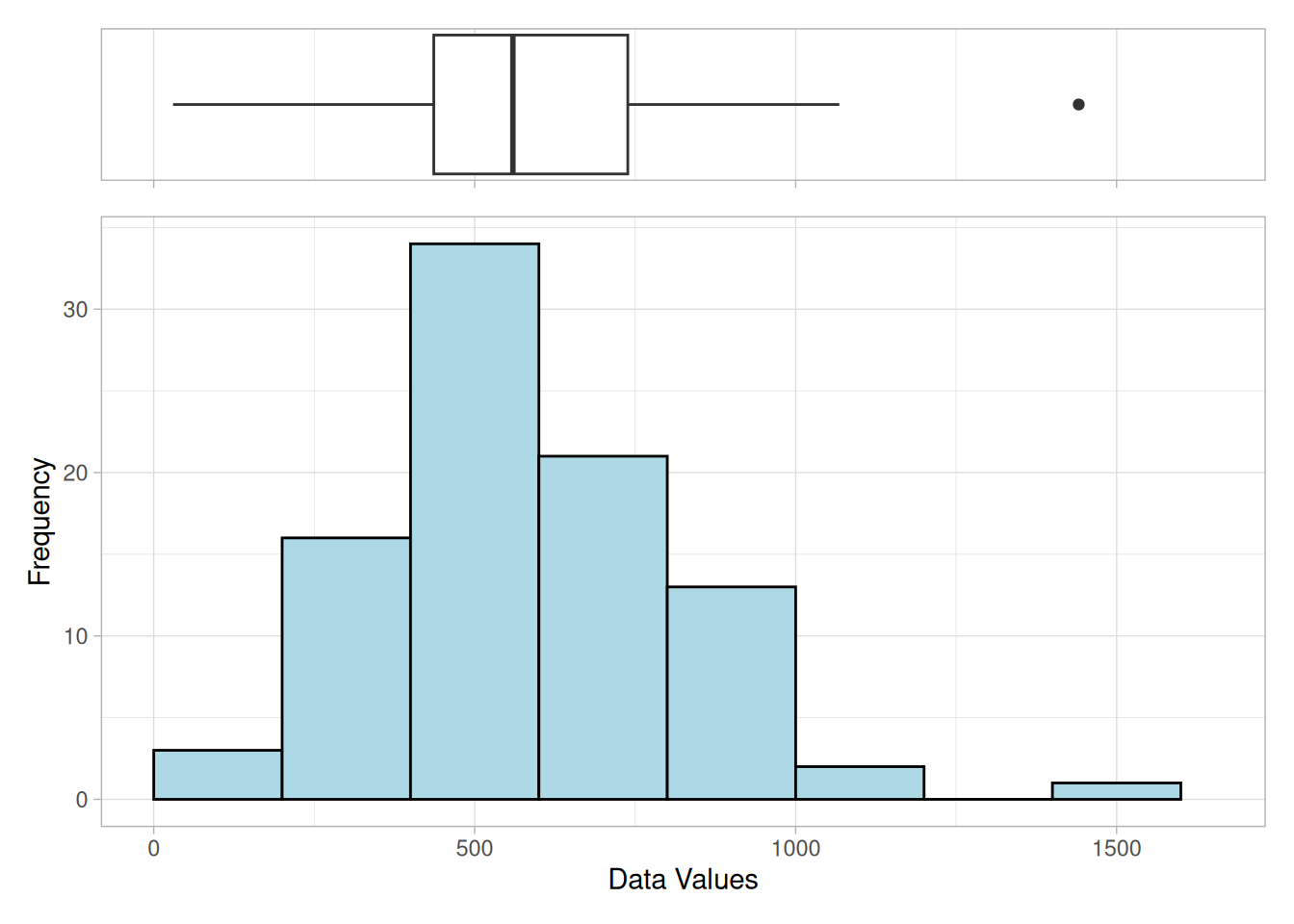

Figure 7.1: Histogram and box plot of the outlier example data

The outlier is identified as the largest value in the data set, 1441, and appears as the circle to the right of the box plot.

Outliers may contain important information

Outliers should be investigated carefully. Often they contain valuable information about the process under investigation or the data gathering and recording process. Before considering the possible elimination of these points from the data, one should try to understand why they appeared and whether it is likely similar values will continue to appear. Of course, outliers are often bad data points.

7.1.7 What are trends in sequential process or product data?

Detecting trends by plotting the data points to see if a line with an obviously non-zero slope fits the points

Detecting trends is equivalent to comparing the process values to what we would expect a series of numbers to look like if there were no trends. If we see a significant departure from a model where the next observation is equally likely to go up or down, then we would reject the hypothesis of “no trend”.

A common way of investigating for trends is to fit a straight line to the data and observe the line’s direction (or slope). If the line looks horizontal, then there is no evidence of a trend; otherwise there is. Formally, this is done by testing whether the slope of the line is significantly different from zero. The methodology for this is covered in Chapter 4.

Other trend tests

A non-parametric approach for detecting significant trends known as the Reverse Arrangement Test is described in Chapter 8.

7.2 Comparisons Based on Data from One Process

Questions answered in this section

For a single process, the current state of the process can be compared with a nominal or hypothesized state. This section outlines techniques for answering the following questions from data gathered from a single process:

1. Do the observations come from a particular distribution?
   1. Chi-Square Goodness-of-Fit test for a continuous or discrete distribution
   2. Kolmogorov-Smirnov test for a continuous distribution
   3. Anderson-Darling and Shapiro-Wilk tests for a continuous distribution
2. Are the data consistent with the assumed process mean?
   1. Confidence interval approach
   2. Sample sizes required
3. Are the data consistent with a nominal standard deviation?
   1. Confidence interval approach
   2. Sample sizes required
4. Does the proportion of defectives meet requirements?
   1. Confidence intervals
   2. Sample sizes required
5. Does the defect density meet requirements?
6. What intervals contain a fixed percentage of the data?
   1. Approximate intervals that contain most of the population values
   2. Percentiles
   3. Tolerance intervals
   4. Tolerance intervals based on the smallest and largest observations

General forms of testing

These questions are addressed either by an hypothesis test or by a confidence interval.

Parametric vs. non-parametric testing

All hypothesis-testing procedures can be broadly described as either parametric or non-parametric/distribution-free. Parametric test procedures are those that:

1. Involve hypothesis testing of specified parameters (such as “the population mean = 50 grams”…).
2. Require a stringent set of assumptions about the underlying sampling distributions.

When to use nonparametric methods?

When do we require non-parametric or distribution-free methods? Here are a few circumstances that may be candidates:

1. The measurements are only categorical; i.e., they are nominally scaled, or ordinally (in ranks) scaled.
2. The assumptions underlying the use of parametric methods cannot be met.
3. The situation at hand requires an investigation of such features as randomness, independence, symmetry, or goodness of fit rather than the testing of hypotheses about specific values of particular population parameters.

Difference between non-parametric and distribution-free

Some authors distinguish between non-parametric and distribution-free procedures.

Distribution-free test procedures are broadly defined as:

1. Those whose test statistic does not depend on the form of the underlying population distribution from which the sample data were drawn, or
2. Those for which the data are nominally or ordinally scaled.

Nonparametric test procedures are defined as those that are not concerned with the parameters of a distribution.

Advantages of nonparametric methods

Distribution-free or nonparametric methods have several advantages, or benefits:

1. They may be used on all types of data – categorical data, which are nominally scaled or are in rank form, called ordinally scaled, as well as interval or ratio-scaled data.
2. For small sample sizes they are easy to apply.
3. They make fewer and less stringent assumptions than their parametric counterparts.
4. Depending on the particular procedure they may be almost as powerful as the corresponding parametric procedure when the assumptions of the latter are met, and when this is not the case, they are generally more powerful.

Disadvantages of nonparametric methods

Of course there are also disadvantages:

1. If the assumptions of the parametric methods can be met, it is generally more efficient to use them.
2. For large sample sizes, data manipulations tend to become more laborious, unless computer software is available.
3. Often special tables of critical values are needed for the test statistic, and these values cannot always be generated by computer software. On the other hand, the critical values for the parametric tests are readily available and generally easy to incorporate in computer programs.

7.2.1 Do the observations come from a particular distribution?

Data are often assumed to come from a particular distribution

Goodness-of-fit tests indicate whether or not it is reasonable to assume that a random sample comes from a specific distribution. Statistical techniques often rely on observations having come from a population that has a distribution of a specific form (e.g., normal, lognormal, Poisson, etc.). Standard control charts for continuous measurements, for instance, require that the data come from a normal distribution. Accurate lifetime modeling requires specifying the correct distributional model. There may be historical or theoretical reasons to assume that a sample comes from a particular population, as well. Past data may have consistently fit a known distribution, for example, or theory may predict that the underlying population should be of a specific form.

Hypothesis Test model for Goodness-of-fit

Goodness-of-fit tests are a form of hypothesis testing where the null and alternative hypotheses are

\(H_0\): Sample data come from the stated distribution.

\(H_a\): Sample data do not come from the stated distribution.

Parameters may be assumed or estimated from the data

One needs to consider whether a simple or composite hypothesis is being tested. For a simple hypothesis, values of the distribution’s parameters are specified prior to drawing the sample. For a composite hypothesis, one or more of the parameters is unknown. Often, these parameters are estimated using the sample observations.

A simple hypothesis would be:

\(H_0\): Data are from a normal distribution, \(\mu=0\) and \(\sigma=1\).

A composite hypothesis would be:

\(H_0\): Data are from a normal distribution, unknown \(\mu\) and \(\sigma\).

Composite hypotheses are more common because they allow us to decide whether a sample comes from any distribution of a specific type. In this situation, the form of the distribution is of interest, regardless of the values of the parameters. Unfortunately, composite hypotheses are more difficult to work with because the critical values are often hard to compute.

Problems with censored data

A second issue that affects a test is whether the data are censored. When data are censored, sample values are in some way restricted. Censoring occurs if the range of potential values are limited such that values from one or both tails of the distribution are unavailable (e.g., right and/or left censoring – where high and/or low values are missing). Censoring frequently occurs in reliability testing, when either the testing time or the number of failures to be observed is fixed in advance. A thorough treatment of goodness-of-fit testing under censoring is beyond the scope of this document. See D’Agostino and Stephens (1986) for more details.

Three types of tests will be covered

Three goodness-of-fit tests are examined in detail:

1. Chi-square test for continuous and discrete distributions;
2. Kolmogorov-Smirnov test for continuous distributions based on the empirical distribution function (EDF);
3. Anderson-Darling test for continuous distributions.

A more extensive treatment of goodness-of-fit techniques is presented in D’Agostino and Stephens (1986). Along with the tests mentioned above, other general and specific tests are examined, including tests based on regression and graphical techniques.

7.2.1.1 Chi-square goodness-of-fit test

Choice of number of groups for “Goodness of Fit” tests is important – but only useful rules of thumb can be given

The test requires that the data first be grouped. The actual number of observations in each group is compared to the expected number of observations and the test statistic is calculated as a function of this difference. The number of groups and how group membership is defined will affect the power of the test (i.e., how sensitive it is to detecting departures from the null hypothesis). Power will not only be affected by the number of groups and how they are defined, but by the sample size and shape of the null and underlying (true) distributions. Despite the lack of a clear “best method”, some useful rules of thumb can be given.

Group Membership

When data are discrete, group membership is unambiguous. Tabulation or cross tabulation can be used to categorize the data. Continuous data present a more difficult challenge. One defines groups by segmenting the range of possible values into non-overlapping intervals. Group membership can then be defined by the endpoints of the intervals. In general, power is maximized by choosing endpoints such that group membership is equiprobable (i.e., the probabilities associated with an observation falling into a given group are divided as evenly as possible across the intervals). Many commercial software packages follow this procedure.

Rule-of-thumb for number of groups

One rule-of-thumb suggests using the value \(2n^{2/5}\) as a good starting point for choosing the number of groups. Another well-known rule-of-thumb requires every group to have at least five data points.

Computation of the chi-square goodness-of-fit test

The formulas for the computation of the chi-square goodness-of-fit test are given in the EDA chapter.

7.2.1.2 Kolmogorov-Smirnov test

The K-S test is a good alternative to the chi-square test

The Kolmogorov-Smirnov (K-S) test was originally proposed in the 1930’s in papers by Kolmogorov (1933) and Smirnov (1936). Unlike the Chi-Square test, which can be used for testing against both continuous and discrete distributions, the K-S test is only appropriate for testing data against a continuous distribution, such as the normal or Weibull distribution. It is one of a number of tests that are based on the empirical cumulative distribution function (ECDF).

Note

NIST’s original page links both the Kolmogorov (1933) and Smirnov (1936) citations to the chapter’s general reference list page rather than to specific entries, and the chapter’s own reference list has no corresponding entries for either paper. We cite Kolmogorov’s “Sulla Determinazione Empirica di una Legge di Distribuzione” (Giornale dell’Istituto Italiano degli Attuari, 1933) and Smirnov’s “Sur la Distribution de \(\omega^2\)” (Comptes Rendus de l’Académie des Sciences, 1936), the papers conventionally credited with introducing the one- and two-sample forms of this test.

K-S procedure

Details on the construction and interpretation of the K-S test statistic, \(D\), and examples for several distributions are outlined in Chapter 1.

The probability associated with the test statistic is difficult to compute

Critical values associated with the test statistic, \(D\), are difficult to compute for finite sample sizes, often requiring Monte Carlo simulation. However, some general purpose statistical software programs support the Kolmogorov-Smirnov test at least for some of the more common distributions. Tabled values can be found in Birnbaum (1952). A correction factor can be applied if the parameters of the distribution are estimated with the same data that are being tested. See D’Agostino and Stephens (1986) for details.

7.2.1.3 Anderson-Darling and Shapiro-Wilk tests

Purpose: Test for distributional adequacy

The Anderson-Darling Test

The Anderson-Darling test (Stephens (1974)) is used to test if a sample of data comes from a specific distribution. It is a modification of the Kolmogorov-Smirnov (K-S) test and gives more weight to the tails of the distribution than does the K-S test. The K-S test is distribution free in the sense that the critical values do not depend on the specific distribution being tested.

Requires critical values for each distribution

The Anderson-Darling test makes use of the specific distribution in calculating critical values. This has the advantage of allowing a more sensitive test and the disadvantage that critical values must be calculated for each distribution. Tables of critical values are not given in this handbook (see Stephens (1974, 1976, 1977a, 1977b, 1979)) because this test is usually applied with a statistical software program that produces the relevant critical values. Currently, Dataplot computes critical values for the Anderson-Darling test for the following distributions:

• normal
• lognormal
• Weibull
• extreme value type I.

Anderson-Darling procedure

Details on the construction and interpretation of the Anderson-Darling test statistic, \(A^2\), and examples for several distributions are outlined in Chapter 1.

Shapiro-Wilk test for normality

The Shapiro-Wilk Test For Normality

The Shapiro-Wilk test, proposed in Shapiro and Wilk (1965), calculates a \(W\) statistic that tests whether a random sample, \(x_1, x_2, \ldots, x_n\) comes from (specifically) a normal distribution. Small values of \(W\) are evidence of departure from normality and percentage points for the \(W\) statistic, obtained via Monte Carlo simulations, were reproduced by Pearson and Hartley (1972, table 16). This test has done very well in comparison studies with other goodness of fit tests.

The \(W\) statistic is calculated as follows:

\[ W = \frac{\left( \sum_{i=1}^n a_i x_{(i)} \right)^2} {\sum_{i=1}^n (x_i - \bar{x})^2} \, , \]

where the \(x_{(i)}\) are the ordered sample values (\(x_{(1)}\) is the smallest) and the \(a_i\) are constants generated from the means, variances and covariances of the order statistics of a sample of size \(n\) from a normal distribution (see Pearson and Hartley (1972, table 15)).

For more information about the Shapiro-Wilk test the reader is referred to the original Shapiro and Wilk (1965) paper and the tables in Pearson and Hartley (1972).

7.2.2 Are the data consistent with the assumed process mean?

The testing of \(H_0\) for a single population mean

Given a random sample of measurements, \(Y_1, \ldots, Y_N\), there are three types of questions regarding the true mean of the population that can be addressed with the sample data. They are:

1. Does the true mean agree with a known standard or assumed mean?
2. Is the true mean of the population less than a given standard?
3. Is the true mean of the population at least as large as a given standard?

Typical null hypotheses

The corresponding null hypotheses that test the true mean, \(\mu\), against the standard or assumed mean, \(\mu_0\), are:

1. \(H_0: \,\, \mu = \mu_0\)
2. \(H_0: \,\, \mu \le \mu_0\)
3. \(H_0: \,\, \mu \ge \mu_0\)

Test statistic where the standard deviation is not known

The basic statistics for the test are the sample mean and the standard deviation. The form of the test statistic depends on whether the population standard deviation, \(\sigma\), is known or is estimated from the data at hand. The more typical case is where the standard deviation must be estimated from the data, and the test statistic is

\[ t = \frac{\bar{Y} - \mu_0}{s/\sqrt{N}} \, , \]

where the sample mean is

\[ \bar{Y} = \frac{1}{N} \sum_{i=1}^N Y_i \, , \]

and the sample standard deviation is

\[ s = \sqrt{\frac{1}{N-1} \sum_{i=1}^N \left( Y_i - \bar{Y}\right)^2} \, , \]

with \(N-1\) degrees of freedom.

Comparison with critical values

For a test at significance level \(\alpha\), where \(\alpha\) is chosen to be small, typically 0.01, 0.05 or 0.10, the hypothesis associated with each case enumerated above is rejected if:

1. \(|t| \ge t_{1-\alpha/2, \, N-1}\)
2. \(t \ge t_{1-\alpha, \, N-1}\)
3. \(t \le t_{\alpha, \, N-1}\)

where \(t_{1-\alpha/2, \, N-1}\) is the \(1-\alpha/2\) critical value from the \(t\) distribution with \(N-1\) degrees of freedom and similarly for cases (2) and (3). Critical values can be found in the \(t\)-table in Chapter 1.

Test statistic where the standard deviation is known

If the standard deviation is known, the form of the test statistic is

\[ z = \frac{\bar{Y} - \mu_0}{\sigma/\sqrt{N}} \, . \]

For case (1), the test statistic is compared with \(z_{1-\alpha/2}\), which is the \(1-\alpha/2\) critical value from the standard normal distribution, and similarly for cases (2) and (3).

Caution

If the standard deviation is assumed known for the purpose of this test, this assumption should be checked by a test of hypothesis for the standard deviation.

An illustrative example of the t-test

The following numbers are particle (contamination) counts for a sample of 10 semiconductor silicon wafers:

50  48  44  56  61  52  53  55  67  51

library(tidyverse)

wafer_counts <- c(50, 48, 44, 56, 61, 52, 53, 55, 67, 51)

tibble(Statistic = c("Mean", "Standard Deviation"), Value = c(mean(wafer_counts), sd(wafer_counts))) |>
  knitr::kable(digits = 3, align = "lr")

Statistic	Value
Mean	53.700
Standard Deviation	6.567

The mean = 53.7 counts and the standard deviation = 6.567 counts.

The test is two-sided

Over a long run the process average for wafer particle counts has been 50 counts per wafer, and on the basis of the sample, we want to test whether a change has occurred. The null hypothesis that the process mean is 50 counts is tested against the alternative hypothesis that the process mean is not equal to 50 counts. The purpose of the two-sided alternative is to rule out a possible process change in either direction.

Critical values

For a significance level of \(\alpha\) = 0.05, the chances of erroneously rejecting the null hypothesis when it is true are 5% or less. (For a review of hypothesis testing basics, see Chapter 1).

Even though there is a history on this process, it has not been stable enough to justify the assumption that the standard deviation is known. Therefore, the appropriate test statistic is the \(t\)-statistic. Substituting the sample mean, sample standard deviation, and sample size into the formula for the test statistic gives a value of

n <- length(wafer_counts)
t_stat <- (mean(wafer_counts) - 50) / (sd(wafer_counts) / sqrt(n))
t_crit <- qt(0.975, n - 1)

tibble(Statistic = c("t", "Degrees of Freedom", "Critical value t(0.975, 9)"), Value = c(t_stat, n - 1, t_crit)) |>
  knitr::kable(digits = 3, align = "lr")

Statistic	Value
t	1.782
Degrees of Freedom	9.000
Critical value t(0.975, 9)	2.262

\[ t = 1.782 \, , \]

with degrees of freedom \(N\) - 1 = 9. This value is tested against the critical value

\[ t_{1-0.025, \, 9} = 2.262 \, , \]

from the \(t\)-table where the critical value is found under the column labeled 0.975 for the probability of exceeding the critical value and in the row for 9 degrees of freedom. The critical value is based on \(\alpha/2\) instead of \(\alpha\) because of the two-sided alternative (two-tailed test) which requires equal probabilities in each tail of the distribution that add to \(\alpha\).

Conclusion

Because the value of the test statistic falls in the interval (-2.262, 2.262), we cannot reject the null hypothesis and, therefore, we may continue to assume the process mean is 50 counts.

7.2.2.1 Confidence interval approach

Testing using a confidence interval

The hypothesis test results in a “yes” or “no” answer. The null hypothesis is either rejected or not rejected. There is another way of testing a mean and that is by constructing a confidence interval about the true but unknown mean.

General form of confidence intervals where the standard deviation is unknown

Tests of hypotheses that can be made from a single sample of data were discussed on the foregoing page. As with null hypotheses, confidence intervals can be two-sided or one-sided, depending on the question at hand. The general form of confidence intervals, for the three cases discussed earlier, where the standard deviation is unknown are:

1. Two-sided confidence interval for \(\mu\):

\[ \bar{Y} + \frac{s}{\sqrt{N}} \, t_{\alpha/2, \, N-1} \, \le \, \mu \, \le \, \bar{Y} + \frac{s}{\sqrt{N}} \, t_{1-\alpha/2, \, N-1} \, , \]

2. Lower one-sided confidence interval for \(\mu\):

\[ \mu \ge \bar{Y} + \frac{s}{\sqrt{N}} \, t_{\alpha, \, N-1} \, , \]

3. Upper one-sided confidence interval for \(\mu\):

\[ \mu \le \bar{Y} + \frac{s}{\sqrt{N}} \, t_{1-\alpha, \, N-1} \, , \]

where \(t_{\alpha/2, \, N-1}\) is the \(\alpha/2\) critical value from the \(t\) distribution with \(N-1\) degrees of freedom and similarly for cases (2) and (3). Critical values can be found in the \(t\) table in Chapter 1.

Confidence level

The confidence intervals are constructed so that the probability of the interval containing the mean is 1 - \(\alpha\). Such intervals are referred to as \(100(1-\alpha)\)% confidence intervals.

A 95% confidence interval for the example

The corresponding confidence interval for the test of hypothesis example on the foregoing page is shown below. A 95% confidence interval for the population mean of particle counts per wafer is given by

library(tidyverse)

wafer_counts <- c(50, 48, 44, 56, 61, 52, 53, 55, 67, 51)
n <- length(wafer_counts)
m <- mean(wafer_counts)
s <- sd(wafer_counts)

lower <- m + s / sqrt(n) * qt(0.025, n - 1)
upper <- m + s / sqrt(n) * qt(0.975, n - 1)

tibble(Bound = c("Lower", "Upper"), Value = c(lower, upper)) |>
  knitr::kable(digits = 1, align = "lr")

Bound	Value
Lower	49.0
Upper	58.4

\[ \begin{aligned} \bar{Y} + \frac{s}{\sqrt{N}} \, (t_{0.025, 9}) \, &\le \, \mu \, \le \, \bar{Y} + \frac{s}{\sqrt{N}} \, (t_{0.975, 9}) \\[0.5em] 53.7 + \frac{6.567}{\sqrt{10}} (-2.262) \, &\le \, \mu \, \le \, 53.7 + \frac{6.567}{\sqrt{10}}(2.262) \\[0.5em] 49.0 \, &\le \, \mu \, \le \, 58.4 \, . \end{aligned} \]

Interpretation

The 95% confidence interval includes the null hypothesis if, and only if, it would be accepted at the 5% level. This interval includes the null hypothesis of 50 counts so we cannot reject the hypothesis that the process mean for particle counts is 50. The confidence interval includes all null hypothesis values for the population mean that would be accepted by an hypothesis test at the 5% significance level. This assumes, of course, a two-sided alternative.

7.2.2.2 Sample sizes required

The computation of sample sizes depends on many things, some of which have to be assumed in advance

Perhaps one of the most frequent questions asked of a statistician is,

“How many measurements should be included in the sample?”

Unfortunately, there is no correct answer without additional information (or assumptions). The sample size required for an experiment designed to investigate the behavior of an unknown population mean will be influenced by the following:

• value selected for \(\alpha\), the risk of rejecting a true hypothesis,
• value of \(\beta\), the risk of accepting a false null hypothesis when a particular value of the alternative hypothesis is true,
• value of the population standard deviation.

Application – estimating a minimum sample size, \(N\), for limiting the error in the estimate of the mean

For example, suppose that we wish to estimate the average daily yield, \(\mu\), of a chemical process by the mean of a sample, \(Y_1, \, \ldots, \, Y_N\), such that the error of estimation is less than \(\delta\) with a probability of 95%. This means that a 95% confidence interval centered at the sample mean should be

\[ \bar{Y} - \delta \le \mu \le \bar{Y} + \delta \, , \]

and if the standard deviation is known,

\[ \delta = \frac{\sigma}{\sqrt{N}} \, z_{1 - 0.025} \, . \]

The critical value from the normal distribution for 1 - \(\alpha\)/2 = 0.975 is 1.96. Therefore,

\[ N \ge \left( \frac{1.96}{\delta} \right)^2 \sigma^2 \, . \]

Limitation and interpretation

A restriction is that the standard deviation must be known. Lacking an exact value for the standard deviation requires some accommodation, perhaps the best estimate available from a previous experiment.

Controlling the risk of accepting a false hypothesis

To control the risk of accepting a false hypothesis, we set not only \(\alpha\), the probability of rejecting the null hypothesis when it is true, but also \(\beta\), the probability of accepting the null hypothesis when in fact the population mean is \(\mu + \delta\) where \(\delta\) is the difference or shift we want to detect.

Standard deviation assumed to be known

The minimum sample size, \(N\), is shown below for two- and one-sided tests of hypotheses with \(\sigma\) assumed to be known.

\[ \begin{aligned} N = (z_{1-\alpha/2} + z_{1-\beta})^2 \left( \frac{\sigma}{\delta} \right)^2 &\rightarrow \text{two-sided test} \\ N = (z_{1-\alpha} + z_{1-\beta})^2 \left( \frac{\sigma}{\delta} \right)^2 &\rightarrow \text{one-sided test} \end{aligned} \]

The quantities \(z_{1-\alpha/2}\) and \(z_{1-\beta}\) are critical values from the normal distribution.

Note that it is usual to state the shift, \(\delta\), in units of the standard deviation, thereby simplifying the calculation.

Example where the shift is stated in terms of the standard deviation

For a one-sided hypothesis test where we wish to detect an increase in the population mean of one standard deviation, the following information is required: \(\alpha\), the significance level of the test, and \(\beta\), the probability of failing to detect a shift of one standard deviation. For a test with \(\alpha\) = 0.05 and \(\beta\) = 0.10, the minimum sample size required for the test is

za <- qnorm(0.95)
zb <- qnorm(0.90)
n_est <- (za + zb)^2

tibble::tibble(Statistic = c("z(0.95)", "z(0.90)", "N"), Value = c(za, zb, n_est)) |>
  knitr::kable(digits = 3, align = "lr")

Statistic	Value
z(0.95)	1.645
z(0.90)	1.282
N	8.564

\[ N = (1.645 + 1.282)^2 = 8.567 \approx 9 \, . \]

More often we must compute the sample size with the population standard deviation being unknown

The procedures for computing sample sizes when the standard deviation is not known are similar to, but more complex, than when the standard deviation is known. The formulation depends on the \(t\) distribution where the minimum sample size is given by

\[ \begin{aligned} N = (t_{1-\alpha/2} + t_{1-\beta})^2 \left( \frac{s}{\delta} \right)^2 &\rightarrow \text{two-sided test} \\ N = (t_{1-\alpha} + t_{1-\beta})^2 \left( \frac{s}{\delta} \right)^2 &\rightarrow \text{one-sided test} \end{aligned} \]

The drawback is that critical values of the \(t\) distribution depend on known degrees of freedom, which in turn depend upon the sample size which we are trying to estimate.

Iterate on the initial estimate using critical values from the \(t\) table

Therefore, the best procedure is to start with an initial estimate based on a sample standard deviation and iterate. Take the example discussed above where the minimum sample size is computed to be \(N\) = 9. This estimate is low. Now use the formula above with degrees of freedom \(N\) - 1 = 8 which gives a second estimate of

ta <- qt(0.95, 8)
tb <- qt(0.90, 8)
n_est2 <- (ta + tb)^2

tibble::tibble(Statistic = c("t(0.95, 8)", "t(0.90, 8)", "N"), Value = c(ta, tb, n_est2)) |>
  knitr::kable(digits = 3, align = "lr")

Statistic	Value
t(0.95, 8)	1.860
t(0.90, 8)	1.397
N	10.604

\[ N = (1.860 + 1.397)^2 = 10.6 \approx 11 \, . \]

It is possible to apply another iteration using degrees of freedom 10, but in practice one iteration is usually sufficient. For the purpose of this example, results have been rounded to the closest integer; however, computer programs for finding critical values from the \(t\) distribution allow non-integer degrees of freedom.

Table showing minimum sample sizes for a two-sided test

The table below gives sample sizes for a two-sided test of hypothesis that the mean is a given value, with the shift to be detected a multiple of the standard deviation. For a one-sided test at significance level \(\alpha\), look under the value of 2\(\alpha\) in column 1. Note that this table is based on the normal approximation (i.e., the standard deviation is known).

library(tidyverse)

alphas <- c(0.01, 0.05, 0.10, 0.20)
betas <- c(0.01, 0.05, 0.10, 0.20, 0.50)
deltas <- c(0.5, 1.0, 1.5)

sample_size_table <- expand_grid(alpha = alphas, beta = betas) |>
  rowwise() |>
  mutate(
    n = list(pmax(ceiling((qnorm(1 - alpha / 2) + qnorm(1 - beta))^2 / deltas^2), 3))
  ) |>
  unnest_wider(n, names_sep = "_") |>
  rename(`delta = 0.5` = n_1, `delta = 1.0` = n_2, `delta = 1.5` = n_3)

sample_size_table |>
  knitr::kable(align = "rrrrr", col.names = c("$\\alpha$", "$\\beta$", "$\\delta = 0.5\\sigma$", "$\\delta = 1.0\\sigma$", "$\\delta = 1.5\\sigma$"))

Table 7.2: Sample size table for two-sided tests

\(\alpha\)	\(\beta\)	\(\delta = 0.5\sigma\)	\(\delta = 1.0\sigma\)	\(\delta = 1.5\sigma\)
0.01	0.01	97	25	11
0.01	0.05	72	18	8
0.01	0.10	60	15	7
0.01	0.20	47	12	6
0.01	0.50	27	7	3
0.05	0.01	74	19	9
0.05	0.05	52	13	6
0.05	0.10	43	11	5
0.05	0.20	32	8	4
0.05	0.50	16	4	3
0.10	0.01	64	16	8
0.10	0.05	44	11	5
0.10	0.10	35	9	4
0.10	0.20	25	7	3
0.10	0.50	11	3	3
0.20	0.01	53	14	6
0.20	0.05	35	9	4
0.20	0.10	27	7	3
0.20	0.20	19	5	3
0.20	0.50	7	3	3

Note

Our recomputed table (using \(N = \lceil (z_{1-\alpha/2} + z_{1-\beta})^2 / \delta^2 \rceil\), floored at a minimum of 3) matches NIST’s published table exactly in 52 of 60 cells. The remaining 8 cells, all in the \(\delta = 0.5\sigma\) column, are smaller than NIST’s value by exactly 1 (e.g., we compute 97 where NIST shows 98 for \(\alpha=\beta=0.01\)). This is consistent with NIST rounding intermediate critical values to fewer decimal places before squaring, which can tip a value just over an integer boundary; it does not affect the other two columns, which match exactly, or the overall use of the table.

7.2.3 Are the data consistent with a nominal standard deviation?

The testing of \(H_0\) for a single population mean

Given a random sample of measurements, \(Y_1, \, \ldots, \, Y_N\), there are three types of questions regarding the true standard deviation of the population that can be addressed with the sample data. They are:

1. Does the true standard deviation agree with a nominal value?
2. Is the true standard deviation of the population less than or equal to a nominal value?
3. Is the true standard deviation of the population at least as large as a nominal value?

Corresponding null hypotheses

The corresponding null hypotheses that test the true standard deviation, \(\sigma\), against the nominal value, \(\sigma_0\), are:

1. \(H_0: \,\, \sigma = \sigma_0\)
2. \(H_0: \,\, \sigma \le \sigma_0\)
3. \(H_0: \,\, \sigma \ge \sigma_0\)

Test statistic

The basic test statistic is the chi-square statistic

\[ \chi^2 = \frac{(N-1)s^2}{\sigma_0^2} \, , \]

with \(N-1\) degrees of freedom where \(s\) is the sample standard deviation; i.e.,

\[ s = \sqrt{\frac{1}{N-1} \sum_{i=1}^N \left( Y_i - \bar{Y} \right)^2} \, . \]

Comparison with critical values

For a test at significance level \(\alpha\), where \(\alpha\) is chosen to be small, typically 0.01, 0.05 or 0.10, the hypothesis associated with each case enumerated above is rejected if:

\[ \begin{aligned} \text{1. } & \chi^2 \ge \chi^2_{1-\alpha/2} \,\, \text{ or } \,\, \chi^2 \le \chi^2_{\alpha/2} \\ \text{2. } & \chi^2 \ge \chi^2_{1-\alpha} \\ \text{3. } & \chi^2 \le \chi^2_{\alpha} \, , \\ \end{aligned} \]

where \(\chi^2_{\alpha/2}\) is the \(\alpha/2\) critical value from the chi-square distribution with \(N-1\) degrees of freedom and similarly for cases (2) and (3). Critical values can be found in the chi-square table in Chapter 1.

Warning

Because the chi-square distribution is a non-negative, asymmetrical distribution, care must be taken in looking up critical values from tables. For two-sided tests, critical values are required for both tails of the distribution.

Example

A supplier of 100 ohm\(\cdot\)cm silicon wafers claims that his fabrication process can produce wafers with sufficient consistency so that the standard deviation of resistivity for the lot does not exceed 10 ohm\(\cdot\)cm. A sample of \(N\) = 10 wafers taken from the lot has a standard deviation of 13.97 ohm\(\cdot\)cm. Is the supplier’s claim reasonable? This question falls under null hypothesis (2) above. For a test at significance level, \(\alpha\) = 0.05, the test statistic,

library(tidyverse)

n <- 10
s <- 13.97
sigma0 <- 10
chisq_stat <- (n - 1) * s^2 / sigma0^2
chisq_crit <- qchisq(0.95, n - 1)

tibble(
  Statistic = c("$\\chi^2$ test statistic", "Critical value $\\chi^2_{0.95,9}$"),
  Value = c(chisq_stat, chisq_crit)
) |>
  knitr::kable(digits = 2, align = "lr")

Statistic	Value
\(\chi^2\) test statistic	17.56
Critical value \(\chi^2_{0.95,9}\)	16.92

\[ \chi^2 = \frac{(N-1)s^2}{\sigma_0^2} = \frac{9(13.97)^2}{100} = 17.56\, , \]

is compared with the critical value, \(\chi_{0.95, \, 9}^2\) = 16.92.

Since the test statistic (17.56) exceeds the critical value (16.92) of the chi-square distribution with 9 degrees of freedom, the manufacturer’s claim is rejected.

7.2.3.1 Confidence interval approach

Confidence intervals for the standard deviation

Confidence intervals for the true standard deviation can be constructed using the chi-square distribution. The \(100(1-\alpha)\)% confidence intervals that correspond to the tests of hypothesis on the previous page are given by

1. Two-sided confidence interval for \(\sigma\)

\[ \frac{s\sqrt{N-1}}{\sqrt{ \chi^2_{1-\alpha/2, N-1} }} \le \sigma \le \frac{s\sqrt{N-1}}{\sqrt{ \chi^2_{\alpha/2, N-1} }} \, ,\]

2. Lower one-sided confidence interval for \(\sigma\)

\[ \sigma \ge \frac{s\sqrt{N-1}}{\sqrt{ \chi^2_{1-\alpha, N-1} }} \, ,\]

3. Upper one-sided confidence interval for \(\sigma\)

\[ 0 \le \sigma \le \frac{s\sqrt{N-1}}{\sqrt{ \chi^2_{\alpha, N-1} }} \, .\]

For case (1), \(\chi_{\alpha/2}^2\) is the \(\alpha/2\) critical value from the chi-square distribution with \(N-1\) degrees of freedom and similarly for cases (2) and (3). Critical values can be found in the chi-square table in Chapter 1.

Choice of risk level \(\alpha\) can change the conclusion

Confidence interval (1) is equivalent to a two-sided test for the standard deviation. That is, if the hypothesized or nominal value, \(\sigma_0\), is not contained within these limits, then the hypothesis that the standard deviation is equal to the nominal value is rejected.

A dilemma of hypothesis testing

A change in \(\alpha\) can lead to a change in the conclusion. This poses a dilemma. What should \(\alpha\) be? Unfortunately, there is no clear-cut answer that will work in all situations. The usual strategy is to set \(\alpha\) small so as to guarantee that the null hypothesis is wrongly rejected in only a small number of cases. The risk, \(\beta\), of failing to reject the null hypothesis when it is false depends on the size of the discrepancy, and also depends on \(\alpha\). The discussion on the next page shows how to choose the sample size so that this risk is kept small for specific discrepancies.

7.2.3.2 Sample sizes required

Sample sizes to minimize risk of false acceptance

The following procedure for computing sample sizes for tests involving standard deviations follows W. Diamond (1989). The idea is to find a sample size that is large enough to guarantee that the risk, \(\beta\), of accepting a false hypothesis is small.

Alternatives are specific departures from the null hypothesis

This procedure is stated in terms of changes in the variance, not the standard deviation, which makes it somewhat difficult to interpret. Tests that are generally of interest are stated in terms of \(\delta\), a discrepancy from the hypothesized variance. For example:

1. Is the true variance larger than its hypothesized value by \(\delta\)?
2. Is the true variance smaller than its hypothesized value by \(\delta\)?

That is, the tests of interest are:

1. \(H_0: \,\, \sigma^2 \ge \sigma_0^2 + \delta ; \,\,\, \delta \ge 0\)
2. \(H_0: \,\, \sigma^2 \le \sigma_0^2 - \delta ; \,\,\, \delta \ge 0\).

Interpretation

The experimenter wants to assure that the probability of erroneously accepting the null hypothesis of unchanged variance is at most \(\beta\). The sample size, \(N\), required for this type of detection depends on the factor, \(\delta\); the significance level, \(\alpha\); and the risk, \(\beta\).

First choose the level of significance and beta risk

The sample size is determined by first choosing appropriate values of \(\alpha\) and \(\beta\) and then following the directions below to find the degrees of freedom, \(\nu\), from the chi-square distribution.

The calculations should be done by creating a table or spreadsheet

First compute

\[ R = 1 + \frac{\delta}{\sigma^2_0} \, . \]

Then generate a table of degrees of freedom, \(\nu\), say between 1 and 200. For case (1) or (2) above, calculate \(\beta_\nu\) and the corresponding value of \(C_\nu\) for each value of degrees of freedom in the table where

\[ \begin{aligned} \text{ 1. } & \beta_\nu & = \chi^2_{1-\alpha, \nu} / R \\ & C_\nu & = \text{Pr }(\chi^2_\nu < \beta_\nu) \\ \text{ 2. } & \beta_\nu & = \chi^2_{\alpha, \nu} / R \\ & C_\nu & = \text{Pr }(\chi^2_\nu > \beta_\nu) \end{aligned} \]

The value of \(\nu\) where \(C_\nu\) is closest to \(\beta\) is the correct degrees of freedom and

\[ N = \nu + 1 \, . \]

Hints on using software packages to do the calculations

The quantity \(\chi_{1-\alpha, \, \nu}^2\) is the critical value from the chi-square distribution with \(\nu\) degrees of freedom which is exceeded with probability \(\alpha\). It is sometimes referred to as the percent point function (PPF) or the inverse chi-square function. The probability that is evaluated to get \(C_\nu\) is called the cumulative density function (CDF).

Example

Consider the case where the variance for resistivity measurements on a lot of silicon wafers is claimed to be 100 (ohm\(\cdot\)cm)\(^2\). A buyer is unwilling to accept a shipment if \(\delta\) is greater than 55 ohm\(\cdot\)cm for a particular lot. This problem falls under case (1) above. How many samples are needed to assure risks of \(\alpha\) = 0.05 and \(\beta\) = 0.01?

Calculations

If software is available to compute the roots (or zero values) of a univariate function, then we can determine the sample size by finding the roots of a function that calculates \(C_\nu\) for a given value of \(\nu\). The procedure is:

1. Define constants.

\[ \begin{aligned} \alpha & = 0.05 \\ \beta & = 0.01 \\ \delta & = 55 \\ \sigma_0^2 & = 100 \\ R & = 1 + \delta / \sigma_0^2 \end{aligned} \]

2. Create a function, \(C_\nu\).

\[ C_\nu = F(F^{-1}(\alpha, \, \nu)/R, \, \nu) - \beta \]

\(F(x, \nu)\) returns the probability of a chi-square random variable with \(\nu\) degrees of freedom that is less than or equal to \(x\) and \(F^{-1}(\alpha, \, \nu)\) returns \(x\) such that \(F(x, \, \nu) = \alpha\).

3. Find the value of \(\nu\) for which the function, \(C_\nu\), is zero.

alpha <- 0.05
beta <- 0.01
delta <- 55
sigma0_sq <- 100
R <- 1 + delta / sigma0_sq

c_nu <- function(nu) pchisq(qchisq(1 - alpha, nu) / R, nu) - beta

nu_root <- uniroot(c_nu, c(100, 200))$root
nu_root

[1] 169.3335

Using this procedure, \(C_\nu\) is zero when \(\nu\) is 169.3. Therefore, the minimum sample size needed to guarantee the risk level is \(N\) = 170.

Alternatively, we can determine the sample size by simply printing computed values of \(C_\nu\) for various values of \(\nu\).

1. Define constants.

\[ \begin{aligned} \alpha & = 0.05 \\ \delta & = 55 \\ \sigma_0^2 & = 100 \\ R & = 1 + \delta / \sigma_0^2 \end{aligned} \]

2. Generate \(C_\nu\) for values of \(\nu\) from 1 to 200.

\[ \beta_\nu = F^{-1}(\alpha, \,\nu) / R\]

\[ C_\nu = F(\beta_\nu, \, \nu) \]

The values of \(C_\nu\) generated for \(\nu\) between 165 and 175 degrees of freedom are shown below.

library(tidyverse)

nu_range <- 165:175
beta_nu <- qchisq(1 - alpha, nu_range) / R
c_nu_vals <- pchisq(beta_nu, nu_range)

tibble(nu = nu_range, beta_nu = beta_nu, C_nu = c_nu_vals) |>
  knitr::kable(digits = 4, align = "rrr", col.names = c("$\\nu$", "$\\beta_\\nu$", "$C_\\nu$"))

Table 7.3: Values of \(C_\nu\) for degrees of freedom 165-175

\(\nu\)	\(\beta_\nu\)	\(C_\nu\)
165	126.4344	0.0114
166	127.1380	0.0110
167	127.8414	0.0107
168	128.5446	0.0104
169	129.2477	0.0101
170	129.9506	0.0098
171	130.6533	0.0095
172	131.3558	0.0092
173	132.0582	0.0090
174	132.7604	0.0087
175	133.4625	0.0085

The value of \(C_\nu\) closest to 0.01 is 0.0101, which is associated with \(\nu\) = 169 degrees of freedom. Therefore, the minimum sample size needed to guarantee the risk level is \(N\) = 170.

7.2.4 Does the proportion of defectives meet requirements?

Testing proportion defective is based on the binomial distribution

The proportion of defective items in a manufacturing process can be monitored using statistics based on the observed number of defectives in a random sample of size \(N\) from a continuous manufacturing process, or from a large population or lot. The proportion defective in a sample follows the binomial distribution where \(p\) is the probability of an individual item being found defective. Questions of interest for quality control are:

1. Is the proportion of defective items within prescribed limits?
2. Is the proportion of defective items less than a prescribed limit?
3. Is the proportion of defective items greater than a prescribed limit?

Hypotheses regarding proportion defective

The corresponding hypotheses that can be tested are:

1. \(p = p_0\)
2. \(p \le p_0\)
3. \(p \ge p_0\)

where \(p_0\) is the prescribed proportion defective.

Note

NIST’s original page states case (1) as \(p \ne p_0\). This is inconsistent with the parallel treatment in Section 7.2.2 and Section 7.2.3, which both state the corresponding two-sided case as a null hypothesis of equality, and with the two-sided rejection region given below (\(|z| \ge z_{1-\alpha/2}\)), which is the test for \(H_0: p = p_0\) against the alternative \(H_a: p \ne p_0\). We give case (1) as \(p = p_0\) to match.

Test statistic based on a normal approximation

Given a random sample of measurements \(Y_1, \, \ldots, \, Y_N\) from a population, the proportion of items that are judged defective from these \(N\) measurements is denoted \(\hat{p}\). The test statistic,

\[ z = \frac{\hat{p} - p_0}{\sqrt{\frac{p_0(1-p_0)}{N}}} \, , \]

depends on a normal approximation to the binomial distribution that is valid for large \(N\), (\(N > 30\)). This approximation simplifies the calculations using critical values from the table of the normal distribution as shown below.

Restriction on sample size

Because the test is approximate, \(N\) needs to be large for the test to be valid. One criterion is that \(N\) should be chosen so that

\[ \text{min }\{ N p_0, \, N(1-p_0)\} \ge 5 \, . \]

For example, if \(p_0\) = 0.1, then \(N\) should be at least 50 and if \(p_0\) = 0.01, then \(N\) should be at least 500. Criteria for choosing a sample size in order to guarantee detecting a change of size \(\delta\) are discussed on another page.

One and two-sided tests for proportion defective

Tests at the \(1-\alpha\) confidence level corresponding to hypotheses (1), (2), and (3) are shown below. For hypothesis (1), the test statistic, \(z\), is compared with \(z_{1-\alpha/2}\), the critical value from the normal distribution that is exceeded with probability \(\alpha/2\) and similarly for (2) and (3). If

1. \(|z| \ge z_{1-\alpha/2}\)
2. \(z \le z_\alpha\)
3. \(z \ge z_{1-\alpha}\)

the null hypothesis is rejected.

Example of a one-sided test for proportion defective

After a new method of processing wafers was introduced into a fabrication process, two hundred wafers were tested, and twenty-six showed some type of defect. Thus, for \(N\) = 200, the proportion defective is estimated to be \(\hat{p}\) = 26/200 = 0.13. In the past, the fabrication process was capable of producing wafers with a proportion defective of at most 0.10. The issue is whether the new process has degraded the quality of the wafers. The relevant test is the one-sided test (3) which guards against an increase in proportion defective from its historical level.

Calculations for a one-sided test of proportion defective

For a test at significance level \(\alpha\) = 0.05, the hypothesis of no degradation is validated if the test statistic \(z\) is less than the critical value, \(z_{0.95}\) = 1.645. The test statistic is computed to be

library(tidyverse)

p_hat <- 26 / 200
p0 <- 0.10
n <- 200

z_stat <- (p_hat - p0) / sqrt(p0 * (1 - p0) / n)
z_crit <- qnorm(0.95)

tibble(Statistic = c("$\\hat{p}$", "z", "Critical value $z_{0.95}$"), Value = c(p_hat, z_stat, z_crit)) |>
  knitr::kable(digits = 3, align = "lr")

Statistic	Value
\(\hat{p}\)	0.130
z	1.414
Critical value \(z_{0.95}\)	1.645

\[ z = \frac{\hat{p} - p_0}{\sqrt{\frac{p_0(1-p_0)}{N}}} = \frac{0.13 - 0.10}{\sqrt{\frac{0.10(0.90)}{200}}} = 1.414 \, . \]

Interpretation

Because the test statistic is less than the critical value (1.645), we cannot reject hypothesis (3) and, therefore, we cannot conclude that the new fabrication method is degrading the quality of the wafers. The new process may, indeed, be worse, but more evidence would be needed to reach that conclusion at the 95% confidence level.

7.2.4.1 Confidence intervals

Confidence intervals using the method of Agresti and Coull

The Wilson method for calculating confidence intervals for proportions (introduced by Wilson (1927), recommended by Brown, Cai and DasGupta (2001) and Agresti and Coull (1998)) is based on inverting the hypothesis test given in Section 7.2.4. That is, solve for the two values of \(p_0\) (say, \(p_{upper}\) and \(p_{lower}\)) that result from setting \(z = z_{1-\alpha/2}\) and solving for \(p_0 = p_{upper}\), and then setting \(z = z_{\alpha/2}\) and solving for \(p_0 = p_{lower}\). (Here, as in Section 7.2.4, \(z_{\alpha/2}\) denotes the variate value from the standard normal distribution such that the area to the left of the value is \(\alpha/2\).) Although solving for the two values of \(p_0\) might sound complicated, the appropriate expressions can be obtained by straightforward but slightly tedious algebra. Such algebraic manipulation isn’t necessary, however, as the appropriate expressions are given in various sources. Specifically, we have

Formulas for the confidence intervals

\[ \begin{aligned} \text{U.L. } & = \frac{\hat{p} + \frac{z^2_{1-\alpha/2}}{2n} + z_{1-\alpha/2} \sqrt{ \frac{\hat{p}(1-\hat{p})}{n} + \frac{z^2_{1-\alpha/2}}{4n^2} }} {1 + \frac{z^2_{1-\alpha/2}}{n}} \\[1em] \text{L.L. } & = \frac{\hat{p} + \frac{z^2_{\alpha/2}}{2n} + z_{\alpha/2} \sqrt{ \frac{\hat{p}(1-\hat{p})}{n} + \frac{z^2_{\alpha/2}}{4n^2} }} {1 + \frac{z^2_{\alpha/2}}{n}} \, . \end{aligned} \]

Procedure does not strongly depend on values of \(p\) and \(n\)

This approach can be substantiated on the grounds that it is the exact algebraic counterpart to the (large-sample) hypothesis test given in section 7.2.4 and is also supported by the research of Agresti and Coull. One advantage of this procedure is that its worth does not strongly depend upon the value of \(n\) and/or \(p\), and indeed was recommended by Agresti and Coull for virtually all combinations of \(n\) and \(p\).

Another advantage is that the lower limit cannot be negative

Another advantage is that the lower limit cannot be negative. That is not true for the confidence expression most frequently used:

\[ \hat{p} \pm z_{1-\alpha/2}\sqrt{\frac{\hat{p}(1-\hat{p})}{n} } \, . \]

A confidence limit approach that produces a lower limit which is an impossible value for the parameter for which the interval is constructed is an inferior approach. This also applies to limits for the control charts that are discussed in Chapter 6.

One-sided confidence intervals

A one-sided confidence interval can also be constructed simply by replacing each \(z_{\alpha/2}\) by \(z_{\alpha}\) in the expression for the lower or upper limit, whichever is desired. The 95% one-sided interval for \(p\) for the example in the preceding section is:

Example

library(tidyverse)

p_hat <- 0.13
n <- 200
z_alpha <- qnorm(0.95)

lower_limit <- (p_hat + z_alpha^2 / (2 * n) - z_alpha * sqrt(p_hat * (1 - p_hat) / n + z_alpha^2 / (4 * n^2))) / (1 + z_alpha^2 / n)

tibble(Statistic = "Lower limit", Value = lower_limit) |>
  knitr::kable(digits = 5, align = "lr")

Statistic	Value
Lower limit	0.09577

\[ \begin{aligned} p & \ge \text{lower limit} \\[0.5em] p & \ge \frac{\hat{p} + \frac{z^2_{\alpha}}{2n} + z_{\alpha} \sqrt{ \frac{\hat{p}(1-\hat{p})}{n} + \frac{z^2_{\alpha}}{4n^2} }} {1 + \frac{z^2_{\alpha}}{n}} \\[0.5em] p & \ge \frac{0.13 + \frac{(-1.645)^2}{2(200)} -1.645 \sqrt{ \frac{0.13(1-0.13)}{200} + \frac{(-1.645)^2}{4(200)^2} }} {1 + \frac{(-1.645)^2}{200}} \\[0.5em] p & \ge 0.09577 \, . \end{aligned} \]

Conclusion from the example

Since the lower bound does not exceed 0.10, in which case it would exceed the hypothesized value, the null hypothesis that the proportion defective is at most 0.10, which was given in the preceding section, would not be rejected if we used the confidence interval to test the hypothesis. Of course a confidence interval has value in its own right and does not have to be used for hypothesis testing.

Exact Intervals for Small Numbers of Failures and/or Small Sample Sizes

Construction of exact two-sided confidence intervals based on the binomial distribution

If the number of failures is very small or if the sample size \(N\) is very small, symmetrical confidence limits that are approximated using the normal distribution may not be accurate enough for some applications. An exact method based on the binomial distribution is shown next. To construct a two-sided confidence interval at the \(100(1-\alpha)\)% confidence level for the true proportion defective \(p\) where \(N_d\) defects are found in a sample of size \(N\) follow the steps below.

1. Solve the equation,

\[ \sum_{k=0}^{N_d} \left( \begin{array}{c} N \\ k \end{array} \right) p_{U}^k (1-p_{U})^{N-k} = \alpha/2 \, , \]

for \(p_U\) to obtain the upper \(100(1-\alpha)\)% limit for \(p\).

2. Next solve the equation,

\[ \sum_{k=0}^{N_d-1} \left( \begin{array}{c} N \\ k \end{array} \right) p_{L}^k (1-p_{L})^{N-k} = 1 - \alpha/2 \, , \]

for \(p_L\) to obtain the lower \(100(1-\alpha)\)% limit for \(p\).

Note

The interval \((p_L, \, p_U)\) is an exact \(100(1-\alpha)\)% confidence interval for \(p\). However, it is not symmetric about the observed proportion defective, \(\hat{p} = N_d/N\).

Binomial confidence interval example

The equations above that determine \(p_L\) and \(p_U\) can be solved using readily available functions. Take as an example the situation where twenty units are sampled from a continuous production line and four items are found to be defective. The proportion defective is estimated to be \(\hat{p}\) = 4/20 = 0.20. The steps for calculating a 90% confidence interval for the true proportion defective, \(p\) follow.

1. Initialize constants.
   alpha = 0.10
   Nd = 4
   N = 20

2. Define a function for upper limit (fu) and a function
   for the lower limit (fl).
   fu = F(Nd, pu, 20) - alpha/2
   fl = F(Nd-1, pl, 20) - (1-alpha/2)

   F is the cumulative density function for the
   binomial distribution.

3. Find the value of pu that corresponds to fu = 0 and
   the value of pl that corresponds to fl = 0 using software
   to find the roots of a function.

alpha <- 0.10
Nd <- 4
N <- 20

fu <- function(p) pbinom(Nd, N, p) - alpha / 2
fl <- function(p) pbinom(Nd - 1, N, p) - (1 - alpha / 2)

pu <- uniroot(fu, c(1e-6, 1 - 1e-6))$root
pl <- uniroot(fl, c(1e-6, 1 - 1e-6))$root

tibble(Statistic = c("$p_U$", "$p_L$"), Value = c(pu, pl)) |>
  knitr::kable(digits = 6, align = "lr")

Statistic	Value
\(p_U\)	0.401030
\(p_L\)	0.071351

The values of \(p_U\) and \(p_L\) for our example are:

pu = 0.401029
pl = 0.071354

Thus, a 90% confidence interval for the proportion defective, \(p\), is (0.071, 0.400). Whether or not the interval is truly “exact” depends on the software.

Terminology Note

Previous versions of the Handbook referred to the method described here as the Agresti-Coull method. However, common practice in the statistics literature is to refer to the method given here as the Wilson method and a similar, but different, method described in Brown, Cai, and DasGupta as the Agresti-Coull method (the Agresti-Coull paper refers to this as the “adjusted Wald” method). We have modified our terminology to be consistent with common practice in the statistical literature.

7.2.4.2 Sample sizes required

Derivation of formula for required sample size when testing proportions

The method of determining sample sizes for testing proportions is similar to the method for determining sample sizes for testing the mean. Although the sampling distribution for proportions actually follows a binomial distribution, the normal approximation is used for this derivation.

Problem formulation

We want to test the hypothesis

\[ H_0: \,\, p = p_0 \] \[ H_a: \,\, p \ne p_0 \]

with \(p\) denoting the proportion of defectives.

Define \(\delta\) as the change in the proportion defective that we are interested in detecting

\[ \delta = | p_1 - p_0|\, . \]

Specify the level of statistical significance and statistical power, respectively, by

\[ P(\text{reject } H_0 \mid H_0 \text{ is true with any } p \ne p_0) \le \alpha \]

\[ P(\text{reject } H_0 \mid H_0 \text{ is false with any } p \le \delta) \le 1-\beta \, . \]

Definition of allowable deviation

If we are interested in detecting a change in the proportion defective of size \(\delta\) in either direction, the corresponding confidence interval for \(p\) can be written as

\[ \hat{p} - \delta \le p \le \hat{p} + \delta \, . \]

Relationship to confidence interval

For a \(100(1-\alpha)\)% confidence interval based on the normal distribution, where \(z_{1 - \alpha/2}\) is the critical value of the normal distribution which is exceeded with probability \(\alpha/2\), is

\[ \delta = z_{1-\alpha/2} \, \sqrt{\frac{p_0 (1-p_0)}{N}} + z_{1-\beta} \, \sqrt{\frac{p_1 (1-p_1)}{N}} \, . \]

Minimum sample size

Thus, the minimum sample size is

1. For a two-sided interval

\[ N \ge \left( \frac{z_{1-\alpha/2} \, \sqrt{p_0 (1-p_0)} + z_{1-\beta} \, \sqrt{p_1 (1-p_1)}}{\delta} \, \right)^2 \, . \]

2. For a one-sided interval

\[ N \ge \left( \frac{z_{1-\alpha} \, \sqrt{p_0 (1-p_0)} + z_{1-\beta} \, \sqrt{p_1 (1-p_1)}}{\delta} \, \right)^2 \, . \]

The mathematical details of this derivation are given on pages 30-34 of Fleiss, Levin, and Paik (2003).

Continuity correction

Fleiss, Levin, and Paik also recommend the following continuity correction,

\[ N = N' + 1/\delta \, , \]

with \(N'\) denoting the sample size computed using the above formula.

Example of calculating sample size for testing proportion defective

Suppose that a department manager needs to be able to detect any change above 0.10 in the current proportion defective of his product line, which is running at approximately 10% defective. He is interested in a one-sided test and does not want to stop the line except when the process has clearly degraded and, therefore, he chooses a significance level for the test of 5%. Suppose, also, that he is willing to take a risk of 10% of failing to detect a change of this magnitude. With these criteria:

1. \(z_{0.95} = 1.645 , \,\, z_{0.90} = 1.282\)
2. \(\delta = 0.10 \,\, (p_1 = 0.20)\)
3. \(p_0 = 0.10\)

and the minimum sample size for a one-sided test procedure is

library(tidyverse)

za <- qnorm(0.95)
zb <- qnorm(0.90)
p0 <- 0.10
p1 <- 0.20
delta <- 0.10

n_min <- ((za * sqrt(p0 * (1 - p0)) + zb * sqrt(p1 * (1 - p1))) / delta)^2
n_cc <- n_min + 1 / delta

tibble(Statistic = c("N (raw)", "N (continuity-corrected)"), Value = c(n_min, n_cc)) |>
  knitr::kable(digits = 1, align = "lr")

Statistic	Value
N (raw)	101.2
N (continuity-corrected)	111.2

\[\begin{aligned} N & \ge \left( \frac{z_{1-\alpha} \, \sqrt{p_0 (1-p_0)} + z_{1-\beta} \, \sqrt{p_1 (1-p_1)}}{\delta} \, \right)^2 \\[0.5em] & = \left( \frac{1.645 \, \sqrt{0.1 \times 0.9} + 1.282 \, \sqrt{0.2 \times 0.8}}{0.1} \, \right)^2 \\[0.5em] & \approx 102 \, . \end{aligned} \]

With the continuity correction, the minimum sample size becomes 112.

7.2.5 Does the defect density meet requirements?

Testing defect densities is based on the Poisson distribution

The number of defects observed in an area of size \(A\) units is often assumed to have a Poisson distribution with parameter \(A \times D\), where \(D\) is the actual process defect density (\(D\) is defects per unit area). In other words:

\[ P(\text{Number of Defects } = n) = \frac{(AD)^n}{n!} e^{-AD} \, . \]

The questions of primary interest for quality control are:

1. Is the defect density within prescribed limits?
2. Is the defect density less than a prescribed limit?
3. Is the defect density greater than a prescribed limit?

Normal approximation to the Poisson

We assume that \(AD\) is large enough so that the normal approximation to the Poisson applies (in other words, \(AD >\) 10 for a reasonable approximation and \(AD >\) 20 for a good one). That translates to

\[ P(\text{Number of Defects } < n) = \Phi \left( \frac{n-AD}{\sqrt{AD}} \right) \, , \]

where \(\Phi\) is the standard normal distribution function.

Test statistic based on a normal approximation

If, for a sample of area \(A\) with a defect density target of \(D_0\), a defect count of \(C\) is observed, then the test statistic,

\[ Z = \frac{C - AD_0}{\sqrt{AD_0}} \, , \]

can be used exactly as shown in the discussion of the test statistic for fraction defectives in the preceding section.

Testing the hypothesis that the process defect density is less than or equal to \(D_0\)

For example, after choosing a sample size of area \(A\) (see below for sample size calculation) we can reject that the process defect density is less than or equal to the target \(D_0\) if the number of defects \(C\) in the sample is greater than \(C_A\), where

\[ C_A = z_{1-\alpha} \sqrt{AD_0} + AD_0 \, , \]

and \(z_{1-\alpha}\) is the \(100(1-\alpha)\) percentile of the standard normal distribution. The test significance level is \(100(1-\alpha)\). For a 90% significance level use \(z_{0.90}\) = 1.282 and for a 95% test use \(z_{0.95}\) = 1.645. \(\alpha\) is the maximum risk that an acceptable process with a defect density at least as low as \(D_0\) “fails” the test.

Choice of sample size (or area) to examine for defects

In order to determine a suitable area \(A\) to examine for defects, you first need to choose an unacceptable defect density level. Call this unacceptable defect density \(D_1 = k D_0\), where \(k >\) 1.

We want to have a probability of less than or equal to \(\beta\) is of “passing” the test (and not rejecting the hypothesis that the true level is \(D_0\) or better) when, in fact, the true defect level is \(D_1\) or worse. Typically \(\beta\) will be 0.2, 0.1 or 0.05. Then we need to count defects in a sample size of area \(A\), where \(A\) is equal to

\[ A = \frac{k}{D_0} \left( \frac{\frac{z_{1-\alpha}} {\sqrt{k}} - z_\beta} {k-1} \right)^2 \, . \]

Example

Suppose the target is \(D_0\) = 4 defects per wafer and we want to verify a new process meets that target. We choose \(\alpha\) = 0.1 to be the chance of failing the test if the new process is as good as \(D_0\) (\(\alpha\) = the Type I error probability or the “producer’s risk”) and we choose \(\beta\) = 0.1 for the chance of passing the test if the new process is as bad as 6 defects per wafer (\(\beta\) = the Type II error probability or the “consumer’s risk”). That means \(z_{1-\alpha}\) = 1.282 and \(z_{\beta}\) = -1.282.

The sample size needed is \(A\) wafers, where

library(tidyverse)

alpha <- 0.1
beta <- 0.1
D0 <- 4
D1 <- 6
k <- D1 / D0

z_1_alpha <- qnorm(1 - alpha)
z_beta <- qnorm(beta)

A <- (k / D0) * ((z_1_alpha / sqrt(k) - z_beta) / (k - 1))^2
A_rounded <- ceiling(A)
C_A <- z_1_alpha * sqrt(A_rounded * D0) + A_rounded * D0

tibble(
  Statistic = c("$z_{1-\\alpha}$", "$z_\\beta$", "A", "A (rounded up)", "$C_A$"),
  Value = c(z_1_alpha, z_beta, A, A_rounded, C_A)
) |>
  knitr::kable(digits = 2, align = "lr")

Statistic	Value
\(z_{1-\alpha}\)	1.28
\(z_\beta\)	-1.28
A	8.13
A (rounded up)	9.00
\(C_A\)	43.69

\[ A = \frac{1.5}{4} \left( \frac{\frac{1.282}{\sqrt{1.5}} - (-1.282)}{k-1} \right) ^ 2 = 8.1 \, , \]

which we round up to 9.

The test criteria is to “accept” that the new process meets target unless the number of defects in the sample of 9 wafers exceeds

\[ C_A = z_{1-\alpha} \sqrt{AD_0} + AD_0 = 1.282 \sqrt{36} + 36 = 43.7 \, . \]

In other words, the reject criteria for the test of the new process is 44 or more defects in the sample of 9 wafers.

Note: Technically, all we can say if we run this test and end up not rejecting is that we do not have statistically significant evidence that the new process exceeds target. However, the way we chose the sample size for this test assures us we most likely would have had statistically significant evidence for rejection if the process had been as bad as 1.5 times the target.

7.2.6 What intervals contain a fixed percentage of the population values?

Observations tend to cluster around the median or mean

Empirical studies have demonstrated that it is typical for a large number of the observations in any study to cluster near the median. In right-skewed data this clustering takes place to the left of (i.e., below) the median and in left-skewed data the observations tend to cluster to the right (i.e., above) the median. In symmetrical data, where the median and the mean are the same, the observations tend to distribute equally around these measures of central tendency.

Various methods

Several types of intervals about the mean that contain a large percentage of the population values are discussed in this section.

• Approximate intervals that contain most of the population values
• Percentiles
• Tolerance intervals for a normal distribution
• Tolerance intervals based on the smallest and largest observations

7.2.6.1 Approximate intervals that contain most of the population values

Empirical intervals

A rule of thumb is that where there is no evidence of significant skewness or clustering, two out of every three observations (67%) should be contained within a distance of one standard deviation of the mean; 90% to 95% of the observations should be contained within a distance of two standard deviations of the mean; 99-100% should be contained within a distance of three standard deviations. This rule can help identify outliers in the data.

Intervals that apply to any distribution

The Bienayme-Chebyshev rule states that regardless of how the data are distributed, the percentage of observations that are contained within a distance of \(k\) standard deviations of the mean is at least \(100(1-1/k^2)\)%.

Exact intervals for the normal distribution

The Bienayme-Chebyshev rule is conservative because it applies to any distribution. For a normal distribution, a higher percentage of the observations are contained within \(k\) standard deviations of the mean as shown in the following table.

library(tidyverse)

tibble(
  k = 1:4,
  `Empirical Rule` = c("67%", "90-95%", "99-100%", "N/A"),
  `Bienayme-Chebyshev` = c("N/A", "at least 75%", "at least 88.89%", "at least 93.75%"),
  `Normal Distribution` = str_c(round((pnorm(1:4) - pnorm(-(1:4))) * 100, 2), "%")
) |>
  knitr::kable(align = "lccc", col.names = c("$k$, No. of Standard Deviations", "Empirical Rule", "Bienayme-Chebyshev", "Normal Distribution"))

Table 7.4: Percentage of observations contained between the mean and k standard deviations

\(k\), No. of Standard Deviations	Empirical Rule	Bienayme-Chebyshev	Normal Distribution
1	67%	N/A	68.27%
2	90-95%	at least 75%	95.45%
3	99-100%	at least 88.89%	99.73%
4	N/A	at least 93.75%	99.99%

7.2.6.2 Percentiles

Definitions of order statistics and ranks

For a series of measurements \(Y_1, \, \ldots, \, Y_N\), denote the data ordered in increasing order of magnitude by \(Y_{[1]}, \, \ldots, \, Y_{[N]}\). These ordered data are called order statistics. If \(Y_{[j]}\) is the order statistic that corresponds to the measurement \(Y_i\), then the rank for \(Y_i\) is \(j\); i.e.,

\[ Y_{[j]} \sim Y_i \,\, \Longrightarrow \,\, r_i = j \, .\]

Definition of percentiles

Order statistics provide a way of estimating proportions of the data that should fall above and below a given value, called a percentile. The \(p\)th percentile is a value, \(Y_{(p)}\), such that at most \((100 p)\)% of the measurements are less than this value and at most \(100(1-p)\)% are greater. The 50th percentile is called the median.

Percentiles split a set of ordered data into hundredths. (Deciles split ordered data into tenths). For example, 70% of the data should fall below the 70th percentile.

Given \(n\) points, the percentile corresponding to the \(i\)-th point is

\[ \frac{i}{n+1} \]

More typically we start with a desired percentile value and this percentile of interest may not correspond to a specific data point. In this case, interpolation between points is required. There is not a standard universally accepted way to perform this interpolation. After describing our default method, several alternative methods are given. All of the methods discussed here are used in practice.

Estimation of percentiles

Percentiles can be estimated from \(N\) measurements as follows: for the \(p\)th percentile, set \(p(N+1)\) equal to \(k + d\) for \(k\) an integer, and \(d\), a fraction greater than or equal to 0 and less than 1.

1. For \(0 \lt k \lt N, \,\,\,\,\, Y_{(p)} = Y_{[k]} + d \left( Y_{[k+1]} - Y_{[k]} \right)\)

2. For \(k = 0, \,\,\,\,\, Y_{(p)} = Y_{[1]}\)

   Note that any \(p \le\) 1/(\(N\)+1) will simply be set to the minimum value.

3. For \(k \ge N, \,\,\,\,\, Y_{(p)} = Y_{[N]}\)

   Note that any \(p \ge\) \(N\)/(\(N\)+1) will simply be set to the maximum value.

Example and interpretation

For the purpose of illustration, twelve measurements from a gage study are shown below. The measurements are resistivities of silicon wafers measured in ohm\(\cdot\)cm.

library(tidyverse)

resistivity <- c(95.1772, 95.1567, 95.1937, 95.1959, 95.1442, 95.0610, 95.1591, 95.1195, 95.1065, 95.0925, 95.1990, 95.1682)

tibble(
  i = seq_along(resistivity),
  Measurement = resistivity,
  `Order stat.` = sort(resistivity),
  Rank = rank(resistivity)
) |>
  knitr::kable(digits = 4, align = "rrrr")

Table 7.5: Resistivity measurements, order statistics, and ranks

i	Measurement	Order stat.	Rank
1	95.1772	95.0610	9
2	95.1567	95.0925	6
3	95.1937	95.1065	10
4	95.1959	95.1195	11
5	95.1442	95.1442	5
6	95.0610	95.1567	1
7	95.1591	95.1591	7
8	95.1195	95.1682	4
9	95.1065	95.1772	3
10	95.0925	95.1937	2
11	95.1990	95.1959	12
12	95.1682	95.1990	8

To find the 90th percentile, \(p(N+1)\) = 0.9(13) = 11.7; \(k\) = 11, and \(d\) = 0.7. From condition (1) above, \(Y_{(90)}\) is estimated to be

y90_r6 <- quantile(resistivity, 0.90, type = 6, names = FALSE)
y90_r6

[1] 95.19807

95.1981 ohm\(\cdot\)cm. This percentile, although it is an estimate from a small sample of resistivities measurements, gives an indication of the percentile for a population of resistivity measurements.

Note that there are other ways of calculating percentiles in common use

Hyndman and Fan (1996) in an American Statistician article evaluated nine different methods (we will refer to these as R1 through R9) for computing percentiles relative to six desirable properties. Their goal was to advocate a “standard” definition for percentiles that would be implemented in statistical software. Although this has not in fact happened, the article does provide a useful summary and evaluation of various methods for computing percentiles. Most statistical and spreadsheet software use one of the methods described in Hyndman and Fan.

The method described above corresponds to method R6 of Hyndman and Fan. This is the default method used by Dataplot.

The method advocated by Hyndman and Fan is R8. For the R8 method, set \(p(N+(1/3)) + (1/3)\) and proceed as above. Note that any \(p \le\) (2/3)/(\(N\)+(1/3)) will be set to the minimum value and any \(p \ge\) (\(N\)-(1/3))/(\(N\)+(1/3)) will be set to the maximum value. Both R and Dataplot can optionally use this method. For the example given above, R8 gives

y90_r8 <- quantile(resistivity, 0.90, type = 8, names = FALSE)
y90_r8

[1] 95.19724

95.1972 (compared to 95.1981) for the 90-th percentile.

Some software packages set \(1 + p(N-1)\) equal to \(k + d\) and then proceed as above. This is method R7 of Hyndman and Fan. This is the method used by Excel and is the default method for R (the R quantile function can optionally use any of the nine methods discussed in Hyndman and Fan). For the example given above, R7 gives

y90_r7 <- quantile(resistivity, 0.90, type = 7, names = FALSE)
y90_r7

[1] 95.19568

95.1957.

The R6, R7, and R8 methods give fairly similar, but not exactly the same (particularly for small samples), results. For most purposes, any of these three methods should be acceptable.

Another method of calculating percentiles (given in some elementary textbooks) starts by calculating \(p N\). If that is not an integer, round up to the next highest integer \(k\) and use \(Y_{[k]}\) as the percentile estimate. If \(p N\) is an integer \(k\), use \(0.5 \left( Y_{[k]} + Y_{[k+1]} \right)\). One of R6, R7, or R8 would typically be preferred to this method.

Definition of Tolerance Interval

An interval covering population percentiles can be interpreted as “covering a proportion \(p\) of the population with a level of confidence, say, 90%.” This is known as a tolerance interval.

7.2.6.3 Tolerance intervals for a normal distribution

Definition of a tolerance interval

A confidence interval covers a population parameter with a stated confidence, that is, a certain proportion of the time. There is also a way to cover a fixed proportion of the population with a stated confidence. Such an interval is called a tolerance interval. The endpoints of a tolerance interval are called tolerance limits. An application of tolerance intervals to manufacturing involves comparing specification limits prescribed by the client with tolerance limits that cover a specified proportion of the population.

Difference between confidence and tolerance intervals

Confidence limits are limits within which we expect a given population parameter, such as the mean, to lie. Statistical tolerance limits are limits within which we expect a stated proportion of the population to lie.

Not related to engineering tolerances

Statistical tolerance intervals have a probabilistic interpretation. Engineering tolerances are specified outer limits of acceptability which are usually prescribed by a design engineer and do not necessarily reflect a characteristic of the actual measurements.

Three types of tolerance intervals

Three types of questions can be addressed by tolerance intervals. Question (1) leads to a two-sided interval; questions (2) and (3) lead to one-sided intervals.

1. What interval will contain \(p\) percent of the population measurements?
2. What interval guarantees that \(p\) percent of population measurements will not fall below a lower limit?
3. What interval guarantees that \(p\) percent of population measurements will not exceed an upper limit?

Tolerance intervals for measurements from a normal distribution

For the questions above, the corresponding tolerance intervals are defined by lower (L) and upper (U) tolerance limits which are computed from a series of measurements \(Y_1, \, \ldots, \, Y_N\):

1. \(Y_L = \bar{Y} - k_2 s; \,\,\, Y_U = \bar{Y} + k_2 s\)
2. \(Y_L = \bar{Y} - k_1 s\)
3. \(Y_U = \bar{Y} + k_1 s\)

where the \(k\) factors are determined so that the intervals cover at least a proportion \(p\) of the population with confidence, \(\alpha\). The value of \(p\) is often referred to as the coverage factor.

Calculation of \(k\) factor for a two-sided tolerance limit for a normal distribution

If the data are from a normally distributed population, an approximate value for the \(k_2\) factor as a function of \(p\) and \(\alpha\) for a two-sided tolerance interval (Howe (1969)) is

\[ k_2 = z_{(1+p)/2} \sqrt{\frac{\nu \left(1 + \frac{1}{N}\right) \, }{\chi^2_{1-\alpha, \, \nu}}} \, , \]

where \(\chi_{1-\alpha, \, \nu}^2\) is the critical value of the chi-square distribution with degrees of freedom \(\nu\) that is exceeded with probability \(\alpha\), and \(z_{(1+p)/2}\) is the critical value of the normal distribution associated with cumulative probability \((1+p)/2\).

The quantity \(\nu\) represents the degrees of freedom used to estimate the standard deviation. Most of the time the same sample will be used to estimate both the mean and standard deviation so that \(\nu = N-1\), but the formula allows for other possible values of \(\nu\).

Guenther’s correction to \(k_2\)

Guenther (1977) recommends the following correction to Howe’s approximation

\[ k_2^{*} = wk_2 \]

where

\[ w = \sqrt{ 1 + \frac{N -3 - \chi^2_{N-1,1 - \alpha} } {2(N+1)^2}} \]

For reasonably large values of \(N\), this correction factor should be close to 1.

n_guenther <- 40
alpha_guenther <- 0.95
w <- sqrt(1 + (n_guenther - 3 - qchisq(alpha_guenther, n_guenther - 1)) / (2 * (n_guenther + 1)^2))
w

[1] 0.9973832

For example, for \(N\) = 40 and \(\alpha\) = 0.95, the correction factor is 0.9972.

Example of calculation

For example, suppose that we take a sample of \(N\) = 43 silicon wafers from a lot and measure their thicknesses in order to find tolerance limits within which a proportion \(p\) = 0.90 of the wafers in the lot fall with confidence \(\alpha\) = 0.99. Since the standard deviation, \(s\), is computed from the sample of 43 wafers, the degrees of freedom are \(\nu = N-1\).

The reader can download the data as a text file.

Use of tables in calculating two-sided tolerance intervals

Values of the \(k_2\) factor as a function of \(p\) and \(\alpha\) are tabulated in some textbooks, such as Dixon and Massey (1969). To use the normal and chi-square tables in this handbook to approximate the \(k_2\) factor, follow the steps outlined below.

1. Calculate: \((1+p)/2 = (1+0.9)/2 = 0.95\) and \(\nu = N-1 = 43 - 1 = 42\).

2. Go to the page describing critical values of the normal distribution. In the summary table under the column labeled 0.95, find

   \(z_{(1+p)/2} = z_{0.95} = 1.645\).

3. Go to the table of lower critical values of the chi-square distribution. Under the column labeled 0.01 in the row labeled degrees of freedom = 42, find

   \(\chi_{1-\alpha, \, \nu}^2 = \chi_{0.01, \, 42}^2 = 23.650\).

4. Calculate

library(tidyverse)

p <- 0.90
alpha <- 0.99
N <- 43
nu <- N - 1

z <- qnorm((1 + p) / 2)
chisq_crit <- qchisq(1 - alpha, nu)
k2 <- z * sqrt(nu * (1 + 1 / N) / chisq_crit)

tibble(Statistic = c("$z_{(1+p)/2}$", "$\\chi^2_{1-\\alpha,\\nu}$", "$k_2$"), Value = c(z, chisq_crit, k2)) |>
  knitr::kable(digits = 3, align = "lr")

Statistic	Value
\(z_{(1+p)/2}\)	1.645
\(\chi^2_{1-\alpha,\nu}\)	23.650
\(k_2\)	2.217

\[ k_2 = z_{(1+p)/2} \sqrt{\frac{\nu \left(1 + \frac{1}{N}\right) \, }{\chi^2_{1-\alpha, \, \nu}}} = 1.645 \sqrt{\frac{42\left(\frac{44}{43}\right)}{23.650}} = 2.217 \, . \]

The tolerance limits are then computed from the sample mean, \(\bar{Y}\), and standard deviation, \(s\), according to case(1).

Important notes

The notation for the critical value of the chi-square distribution can be confusing. Values as tabulated are, in a sense, already squared; whereas the critical value for the normal distribution must be squared in the formula above.

Some software is capable of computing a tolerance intervals for a given set of data so that the user does not need to perform all the calculations. In addition, R software is capable of computing an exact value of the \(k_2\) factor thus replacing the approximation given above.

Calculation of a one-sided tolerance interval for a normal distribution

The calculation of an approximate \(k\) factor for one-sided tolerance intervals comes directly from the following set of formulas (Natrella (1963)):

\[ \begin{aligned} k_{1} & = \frac{z_{p} + \sqrt{z_{p}^2 - ab}} {a} \\ a & = 1 - \frac{z_{\alpha}^2}{2(N-1)} \\ b & = z_{p}^2 - \frac{ z_{\alpha}^2}{N} \, . \end{aligned} \]

A one-sided tolerance interval example

For the example above, it may also be of interest to guarantee with 0.99 probability (or 99% confidence) that 90% of the wafers have thicknesses less than an upper tolerance limit. This problem falls under case (3). The calculations for the \(k_1\) factor for a one-sided tolerance interval are:

zp <- qnorm(p)
za <- qnorm(alpha)

a <- 1 - za^2 / (2 * (N - 1))
b <- zp^2 - za^2 / N
k1 <- (zp + sqrt(zp^2 - a * b)) / a

tibble(Statistic = c("a", "b", "$k_1$"), Value = c(a, b, k1)) |>
  knitr::kable(digits = 4, align = "lr")

Statistic	Value
a	0.9356
b	1.5165
\(k_1\)	1.8752

\[ \begin{aligned} a & = 1 - \frac{1}{2(43-1)} \, (2.3263)^2 = 0.9356\\ b & = (1.2816)^2 - \frac{1}{43} \, (2.3263)^2 = 1.5165\\ k_{1} & = \frac{1.2816 + \sqrt{(1.2816)^2 - (0.9356)(1.5165)}} {0.9356} = 1.8752 \, . \end{aligned} \]

Tolerance factor based on the non-central \(t\) distribution

The value of \(k_1\) can also be computed using the inverse cumulative distribution function for the non-central \(t\) distribution. This method may give more accurate results for small values of \(N\). The value of \(k_1\) using the non-central \(t\) distribution (using the same example as above) is:

delta <- zp * sqrt(N)
t_crit <- qt(alpha, N - 1, ncp = delta)
k1_nt <- t_crit / sqrt(N)

tibble(Statistic = c("$\\delta$", "$t_{\\alpha,N-1,\\delta}$", "$k_1$"), Value = c(delta, t_crit, k1_nt)) |>
  knitr::kable(digits = 4, align = "lr")

Statistic	Value
\(\delta\)	8.4037
\(t_{\alpha,N-1,\delta}\)	12.2883
\(k_1\)	1.8740

\[ \begin{aligned} \delta & = z_{p} \sqrt{N} = 1.2816 \sqrt{43} = 8.4037 \\ k_1 & = \frac{ t_{\alpha, \, N-1, \, \delta} }{ \sqrt{N} } = \frac{12.28834}{\sqrt{43}} = 1.8740 \, , \end{aligned} \]

where \(\delta\) is the non-centrality parameter.

In this case, the difference between the two computations is negligible (1.8752 versus 1.8740). However, the difference becomes more pronounced as the value of \(N\) gets smaller (in particular, for \(N \le\) 10). For example, if \(N\) = 43 is replaced with \(N\) = 6, the non-central \(t\) method returns a value of

N6 <- 6

a6 <- 1 - za^2 / (2 * (N6 - 1))
b6 <- zp^2 - za^2 / N6
k1_natrella_6 <- (zp + sqrt(zp^2 - a6 * b6)) / a6

delta6 <- zp * sqrt(N6)
t_crit6 <- qt(alpha, N6 - 1, ncp = delta6)
k1_nt_6 <- t_crit6 / sqrt(N6)

tibble(Method = c("Non-central $t$", "Natrella formulas"), `$k_1$ ($N=6$)` = c(k1_nt_6, k1_natrella_6)) |>
  knitr::kable(digits = 4, align = "lr")

Method	\(k_1\) (\(N=6\))
Non-central \(t\)	4.4111
Natrella formulas	5.2808

4.4111 for \(k_1\) while the method based on the Natrella formulas returns a value of 5.2808.

The disadvantage of the non-central \(t\) method is that it depends on the inverse cumulative distribution function for the non-central \(t\) distribution. This function is not available in many statistical and spreadsheet software programs, but it is available in Dataplot and R. In addition, the inverse of the non-central t function may lose accuracy for large sample sizes. The Natrella formulas only depend on the inverse cumulative distribution function for the normal distribution (which is available in just about all statistical and spreadsheet software programs). Unless you have small samples (say \(N \le\) 10), the difference in the methods should not have much practical effect.

7.2.6.4 Tolerance intervals based on the largest and smallest observations

Tolerance intervals can be constructed for a distribution of any form

The methods on the previous pages for computing tolerance limits are based on the assumption that the measurements come from a normal distribution. If the distribution is not normal, tolerance intervals based on this assumption will not provide coverage for the intended proportion \(p\) of the population. However, there are methods for achieving the intended coverage if the form of the distribution is not known, but these methods may produce substantially wider tolerance intervals.

Risks associated with making assumptions about the distribution

There are situations where it would be particularly dangerous to make unwarranted assumptions about the exact shape of the distribution, for example, when testing the strength of glass for airplane windshields where it is imperative that a very large proportion of the population fall within acceptable limits.

Tolerance intervals based on largest and smallest observations

One obvious choice for a two-sided tolerance interval for an unknown distribution is the interval between the smallest and largest observations from a sample of \(Y_1, \, \ldots, \, Y_N\) measurements. Given the sample size \(N\) and coverage \(p\), an equation from Hahn and Meeker (1991, 91),

\[ \alpha = 1 - Np^{N-1} + (N-1)p^{N} \, , \]

allows us to calculate the confidence \(\alpha\) of the tolerance interval. For example, the confidence levels for selected coverages between 0.5 and 0.9999 are shown below for \(N\) = 25.

library(tidyverse)

N <- 25
coverages <- c(0.5, 0.75, 0.9, 0.95, 0.975, 0.99, 0.995, 0.999, 0.9995, 0.9999)

tibble(
  Coverage = coverages,
  Confidence = 1 - N * coverages^(N - 1) + (N - 1) * coverages^N
) |>
  knitr::kable(digits = 4, align = "rr")

Table 7.6: Confidence vs. coverage for N = 25

Coverage	Confidence
0.5000	1.0000
0.7500	0.9930
0.9000	0.7288
0.9500	0.3576
0.9750	0.1286
0.9900	0.0258
0.9950	0.0069
0.9990	0.0003
0.9995	0.0001
0.9999	0.0000

Note that if 99% confidence is required, the interval that covers the entire sample data set is guaranteed to achieve a coverage of only 75% of the population values.

What is the optimal sample size?

Another question of interest is, “How large should a sample be so that one can be assured with probability \(\alpha\) that the tolerance interval will contain at least a proportion \(p\) of the population?”

Approximation for \(N\)

A rather good approximation for the required sample size is given by

\[ N \cong \frac{1}{4} \frac{(1+p)}{(1-p)} \, \chi^2_{\alpha, \, 4} +\frac{1}{2} \, , \]

where \(\chi_{\alpha, \, 4}^2\) is the critical value of the chi-square distribution with 4 degrees of freedom that is exceeded with probability \(\alpha\).

Example of the effect of \(p\) on the sample size

Suppose we want to know how many measurements to make in order to guarantee that the interval between the smallest and largest observations covers a proportion \(p\) of the population with probability \(\alpha\) = 0.95. From the table for the upper critical value of the chi-square distribution, look under the column labeled 0.95 in the row for 4 degrees of freedom. The value is found to be \(\chi_{0.95, \, 4}^2\) = 9.488 and calculations are shown below for \(p\) equal to 0.90 and 0.99.

chisq_95_4 <- qchisq(0.95, 4)

tibble(
  p = c(0.90, 0.99),
  N = 0.25 * (1 + c(0.90, 0.99)) / (1 - c(0.90, 0.99)) * chisq_95_4 + 0.5
) |>
  knitr::kable(digits = 2, align = "rr")

p	N
0.90	45.57
0.99	472.51

For \(p\) = 0.90, \(\alpha\) = 0.95;

\[ N \cong \frac{1}{4} \frac{(1+0.90)}{(1-0.90)} \, \chi^2_{0.95, 4} + \frac{1}{2} = 0.25(19)(9.488)+0.5 = 45.57 = 46 \, . \]

For \(p\) = 0.99, \(\alpha\) = 0.95;

\[ N \cong \frac{1}{4} \frac{(1+0.99)}{(1-0.99)} \, \chi^2_{0.95, 4} +\frac{1}{2} = 0.25(199)(9.488)+0.5 = 472.5 = 473 \, . \]

These calculations demonstrate that requiring the tolerance interval to cover a very large proportion of the population may lead to an unacceptably large sample size.

7.3 Comparisons Based on Data from Two Processes

Outline for this section

In many manufacturing environments it is common to have two or more processes performing the same task or generating similar products. The following pages describe tests covering several of the most common and useful cases for two processes.

1. Do two processes have the same mean?
   1. Tests when the standard deviations are equal
   2. Tests when the standard deviations are unequal
   3. Tests for paired data
2. Do two processes have the same standard deviation?
3. Do two processes produce the same proportion of defectives?
4. If the observations are failure times, are the failure rates (or mean times to failure) the same?
5. Do two arbitrary processes have the same central tendency?

Example of a dual track process

For example, in an automobile manufacturing plant, there may exist several assembly lines producing the same part. If one line goes down for some reason, parts can still be produced and production will not be stopped. For example, if the parts are piston rings for a particular model car, the rings produced by either line should conform to a given set of specifications.

How does one confirm that the two processes are in fact producing rings that are similar? That is, how does one determine if the two processes are similar?

The goal is to determine if the two processes are similar

In order to answer this question, data on piston rings are collected for each process. For example, on a particular day, data on the diameters of ten piston rings from each process are measured over a one-hour time frame.

To determine if the two processes are similar, we are interested in answering the following questions:

1. Do the two processes produce piston rings with the same diameter?
2. Do the two processes have similar variability in the diameters of the rings produced?

Unknown standard deviation

The second question assumes that one does not know the standard deviation of either process and therefore it must be estimated from the data. This is usually the case, and the tests in this section assume that the population standard deviations are unknown.

Assumption of a normal distribution

The statistical methodology used (i.e., the specific test to be used) to answer these two questions depends on the underlying distribution of the measurements. The tests in this section assume that the data are normally distributed.

7.3.1 Do two processes have the same mean?

Testing hypotheses related to the means of two processes

Given two random samples of measurements,

\[ Y_1, \, \ldots, \, Y_N \,\,\,\,\, \text{ and } \,\,\,\,\, Z_1, \, \ldots, \, Z_N \]

from two independent processes (the \(Y\) values are sampled from process 1 and the \(Z\) values are sampled from process 2), there are three types of questions regarding the true means of the processes that are often asked. They are:

1. Are the means from the two processes the same?
2. Is the mean of process 1 less than or equal to the mean of process 2?
3. Is the mean of process 1 greater than or equal to the mean of process 2?

Typical null hypotheses

The corresponding null hypotheses that test the true mean of the first process, \(\mu_1\), against the true mean of the second process, \(\mu_2\), are:

1. \(H_0: \mu_1 = \mu_2\)
2. \(H_0: \mu_1 \le \mu_2\)
3. \(H_0: \mu_1 \ge \mu_2\)

Note that as previously discussed, our choice of which null hypothesis to use is typically made based on one of the following considerations:

1. When we are hoping to prove something new with the sample data, we make that the alternative hypothesis, whenever possible.
2. When we want to continue to assume a reasonable or traditional hypothesis still applies, unless very strong contradictory evidence is present, we make that the null hypothesis, whenever possible.

Basic statistics from the two processes

The basic statistics for the test are the sample means

\[ \bar{Y} = \frac{1}{N_1} \sum_{i=1}^{N_1} Y_i \, , \,\,\,\,\, \bar{Z} = \frac{1}{N_2} \sum_{i=1}^{N_2} Z_i \]

and the sample standard deviations

\[ s_1 = \sqrt{\frac{\sum_{i=1}^{N_1} (Y_i - \bar{Y})^2}{N_1-1}} \]

\[ s_2 = \sqrt{\frac{\sum_{i=1}^{N_2} (Z_i - \bar{Z})^2}{N_2-1}} \]

with degrees of freedom \(\nu_1 = N_1 - 1\) and \(\nu_2 = N_2 - 1\) respectively.

Form of the test statistic where the two processes have equivalent standard deviations

If the standard deviations from the two processes are equivalent, and this should be tested before this assumption is made, the test statistic is

\[ t = \frac{\bar{Y} - \bar{Z}}{s \sqrt{\frac{1}{N_1} + \frac{1}{N_2}}} \, , \]

where the pooled standard deviation is estimated as

\[ s = \sqrt{\frac{(N_1 - 1) s_1^2 + (N_2 - 1) s_2^2} {(N_1 - 1) + (N_2 - 1)}} \, , \]

with degrees of freedom \(\nu = N_1 + N_2 - 2\).

Form of the test statistic where the two processes do NOT have equivalent standard deviations

If it cannot be assumed that the standard deviations from the two processes are equivalent, the test statistic is

\[ t = \frac{\bar{Y} - \bar{Z}} {\sqrt{\frac{s_1^2}{N_1} + \frac{s_2^2}{N_2}}} \, . \]

The degrees of freedom are not known exactly but can be estimated using the Welch-Satterthwaite approximation

\[ \nu = \frac{\left( \frac{s_1^2}{N_1} + \frac{s_2^2}{N_2} \right)^2} {\frac{s_1^4}{N_1^2(N_1-1)} + \frac{s_2^4}{N_2^2(N_2-1)}} \, . \]

Test strategies

The strategy for testing the hypotheses under (1), (2) or (3) above is to calculate the appropriate \(t\) statistic from one of the formulas above, and then perform a test at significance level \(\alpha\), where \(\alpha\) is chosen to be small, typically .01, .05 or .10. The hypothesis associated with each case enumerated above is rejected if:

1. \(|t| \ge t_{1-\alpha/2, \, \nu}\)
2. \(t \ge t_{1-\alpha, \, \nu}\)
3. \(t \le t_{\alpha, \, \nu}\)

Explanation of critical values

The critical values from the \(t\) table depend on the significance level and the degrees of freedom in the standard deviation. For hypothesis (1), \(t_{1-\alpha/2, \, \nu}\) is the \(1-\alpha/2\) critical value from the \(t\) table with \(\nu\) degrees of freedom and similarly for hypotheses (2) and (3).

Example of unequal number of data points

A new procedure (process 2) to assemble a device is introduced and tested for possible improvement in time of assembly. The question being addressed is whether the mean, \(\mu_2\), of the new assembly process is smaller than the mean, \(\mu_1\), for the old assembly process (process 1). We choose to test hypothesis (2) in the hope that we will reject this null hypothesis and thereby feel we have a strong degree of confidence that the new process is an improvement worth implementing. Data (in minutes required to assemble a device) for both the new and old processes are listed below along with their relevant statistics.

        Device    Process 1 (Old)  Process 2 (New)

           1            32            36
           2            37            31
           3            35            30
           4            28            31
           5            41            34
           6            44            36
           7            35            29
           8            31            32
           9            34            31
          10            38
          11            42

library(tidyverse)

process1_old <- c(32, 37, 35, 28, 41, 44, 35, 31, 34, 38, 42)
process2_new <- c(36, 31, 30, 31, 34, 36, 29, 32, 31)

tibble(
  Statistic = c("Mean", "Standard deviation", "No. measurements", "Degrees freedom"),
  `Process 1 (Old)` = c(mean(process1_old), sd(process1_old), length(process1_old), length(process1_old) - 1),
  `Process 2 (New)` = c(mean(process2_new), sd(process2_new), length(process2_new), length(process2_new) - 1)
) |>
  knitr::kable(digits = 4, align = "lrr")

Statistic	Process 1 (Old)	Process 2 (New)
Mean	36.0909	32.2222
Standard deviation	4.9082	2.5386
No. measurements	11.0000	9.0000
Degrees freedom	10.0000	8.0000

Computation of the test statistic

From this table we generate the test statistic

n1 <- length(process1_old)
n2 <- length(process2_new)
s1 <- sd(process1_old)
s2 <- sd(process2_new)

t_stat <- (mean(process1_old) - mean(process2_new)) / sqrt(s1^2 / n1 + s2^2 / n2)
nu <- (s1^2 / n1 + s2^2 / n2)^2 / (s1^4 / (n1^2 * (n1 - 1)) + s2^4 / (n2^2 * (n2 - 1)))

tibble(Statistic = c("t", "$\\nu$ (Welch-Satterthwaite)"), Value = c(t_stat, nu)) |>
  knitr::kable(digits = 2, align = "lr")

Statistic	Value
t	2.27
\(\nu\) (Welch-Satterthwaite)	15.53

\[ t = \frac{\bar{Y} - \bar{Z}}{\sqrt{s_1^2/N_1 + s_2^2/N_2}} = \frac{36.0909 - 32.2222}{\sqrt{4.9082^2 / 11 + 2.5386^2 / 9}} = 2.2694 \, , \]

with the degrees of freedom approximated by

\[ \nu = \frac{\left( s_1^2 / N_1 + s_2^2 / N_2 \right)^2} {s_1^4 / (N_1^2(N_1-1)) + s_2^4 / (N_2^2(N_2-1))} = \frac{\left( 4.9082^2 / 11 + 2.5386^2 / 9\right)^2} {4.9082^4 / 1210 + 2.5386^4 /648} = 15.5 \, . \]

Decision process

For a one-sided test at the 5% significance level, go to the \(t\) table for 0.95 significance level, and look up the critical value for degrees of freedom \(\nu\) = 16. The critical value is 1.746. Thus, hypothesis (2) is rejected because the test statistic (\(t\) = 2.269) is greater than 1.746 and, therefore, we conclude that process 2 has improved assembly time (smaller mean) over process 1.

7.3.1.1 Analysis of paired observations

Definition of paired comparisons

Given two random samples,

\[ Y_1, \, \ldots, \, Y_N \,\,\,\,\, \text{ and } \,\,\,\,\, Z_1, \, \ldots, \, Z_N \]

from two populations, the data are said to be paired if the \(i\)-th measurement on the first sample is naturally paired with the \(i\)-th measurement on the second sample. For example, if \(N\) supposedly identical products are chosen from a production line, and each one, in turn, is tested with first one measuring device and then with a second measuring device, it is possible to decide whether the measuring devices are compatible; i.e., whether there is a difference between the two measurement systems. Similarly, if “before” and “after” measurements are made with the same device on \(N\) objects, it is possible to decide if there is a difference between “before” and “after”; for example, whether a cleaning process changes an important characteristic of an object. Each “before” measurement is paired with the corresponding “after” measurement, and the differences,

\[ d_i = Y_i - Z_i \,\,\,\,\, (i = 1, \, \ldots, \, N) \, , \]

are calculated.

Basic statistics for the test

The mean and standard deviation for the differences are calculated as

\[ \bar{d} = \frac{1}{N} \sum_{i=1}^N d_i \]

and

\[ s_d = \sqrt{\frac{1}{N-1} \sum_{i=1}^N (d_i - \bar{d})^2} \]

with \(\nu = N-1\) degrees of freedom.

Test statistic based on the \(t\) distribution

The paired-sample \(t\) test is used to test for the difference of two means before and after a treatment. The test statistic is:

\[ t = \frac{\bar{d}}{s_d / \sqrt{N}} \, . \]

The hypotheses described on the foregoing page are rejected if:

1. \(|t| \ge t_{1-\alpha/2, \, \nu}\)
2. \(t \ge t_{1-\alpha, \, \nu}\)
3. \(t \le t_{\alpha, \, \nu}\)

where for hypothesis (1), \(t_{1-\alpha/2, \, \nu}\) is the \(1-\alpha/2\) critical value from the \(t\) distribution with \(\nu\) degrees of freedom and similarly for cases (2) and (3). Critical values can be found in the \(t\) table in Chapter 1.

7.3.1.2 Confidence intervals for differences between means

Definition of confidence interval for difference between population means

Given two random samples,

\[ Y_1, \, \ldots, \, Y_N \,\,\,\,\, \text{ and } \,\,\,\,\, Z_1, \, \ldots, \, Z_N \]

from two populations, two-sided confidence intervals with \(100(1-\alpha)\)% coverage for the difference between the unknown population means, \(\mu_1\) and \(\mu_2\), are shown in the table below. Relevant statistics for paired observations and for unpaired observations are shown elsewhere.

Two-sided confidence intervals with \(100(1-\alpha)\)% coverage for \(\mu_1 - \mu_2\):

Paired observations

\(\mu_1 - \mu_2\) (where \(\sigma_1 = \sigma_2\))

\(\bar{d} \pm t_{1-\alpha/2, \, N-1} \dfrac{s_{d}}{\sqrt{N}}\)

Unpaired observations

\(\mu_1 - \mu_2\) (where \(\sigma_1 = \sigma_2\))	\(\bar{Y} - \bar{Z} \pm t_{1-\alpha/2, \, N_1 + N_2 - 2} \,\, s \sqrt{\dfrac{1}{N_1} + \dfrac{1}{N_2}}\)
\(\mu_1 - \mu_2\) (where \(\sigma_1 \ne \sigma_2\))	\(\bar{Y} - \bar{Z} \pm t_{1-\alpha/2, \, \nu} \, \sqrt{\dfrac{s_{1}^{2}}{N_1} + \dfrac{s_{2}^{2}}{N_2}}\)

Note

NIST’s original page gives the degrees of freedom for the unequal-variance (unpaired) case as \(N_1 + N_2 - 2\), the same value used in the row immediately above it for the equal-variance case. This cannot be correct: the whole point of the unequal-variance case, as developed on the preceding page, is that the degrees of freedom are not known exactly and must be estimated by the Welch-Satterthwaite approximation, \(\nu\). We give the confidence interval here using \(\nu\) (matching the archived page’s own image alt text, “effective df”, which the live page’s rendered formula did not match).

Interpretation of confidence interval

One interpretation of the confidence interval for means is that if zero is contained within the confidence interval, the two population means are equivalent.

7.3.2 Do two processes have the same standard deviation?

Testing hypotheses related to standard deviations from two processes

Given two random samples of measurements,

\[ Y_1, \, \ldots, \, Y_N \,\,\,\,\, \text{ and } \,\,\,\,\, Z_1, \, \ldots, \, Z_N \]

from two independent processes, there are three types of questions regarding the true standard deviations of the processes that can be addressed with the sample data. They are:

1. Are the standard deviations from the two processes the same?
2. Is the standard deviation of one process less than the standard deviation of the other process?
3. Is the standard deviation of one process greater than the standard deviation of the other process?

Typical null hypotheses

The corresponding null hypotheses that test the true standard deviation of the first process, \(\sigma_1\), against the true standard deviation of the second process, \(\sigma_2\), are:

1. \(H_0: \sigma_1 = \sigma_2\)
2. \(H_0: \sigma_1 \le \sigma_2\)
3. \(H_0: \sigma_1 \ge \sigma_2\)

Basic statistics from the two processes

The basic statistics for the test are the sample variances

\[ s_1^2 = \frac{1}{N_1 - 1} \sum_{i=1}^{N_1} (Y_i - \bar{Y})^2 \]

\[ s_2^2 = \frac{1}{N_2 - 1} \sum_{i=1}^{N_2} (Z_i - \bar{Z})^2 \]

and degrees of freedom \(\nu_1 = N_1 - 1\) and \(\nu_2 = N_2 - 1\), respectively.

Form of the test statistic

The test statistic is

\[ F = \frac{s_1^2}{s_2^2} \, . \]

Test strategies

The strategy for testing the hypotheses under (1), (2) or (3) above is to calculate the \(F\) statistic from the formula above, and then perform a test at significance level \(\alpha\), where \(\alpha\) is chosen to be small, typically 0.01, 0.05 or 0.10. The hypothesis associated with each case enumerated above is rejected if:

\[ \begin{array}{cl} 1. & F \le \frac{1}{F_{\alpha/2, \, \nu_2, \, \nu_1}} \text{ or } F \ge F_{\alpha/2, \, \nu_1, \, \nu_2} \\ 2. & F \ge F_{\alpha, \, \nu_1, \, \nu_2} \\ 3. & F \le \frac{1}{F_{\alpha, \, \nu_2, \, \nu_1}} \end{array} \]

Explanation of critical values

The critical values from the \(F\) table depend on the significance level and the degrees of freedom in the standard deviations from the two processes. For hypothesis (1):

• \(F_{\alpha/2, \, \nu_2, \, \nu_1}\) is the upper critical value from the F table with
• \(\nu_2 = N_2-1\) degrees of freedom for the numerator and
• \(\nu_1 = N_1-1\) degrees of freedom for the denominator,

and

• \(F_{\alpha/2, \, \nu_1, \, \nu_2}\) is the upper critical value from the F table with
• \(\nu_1 = N_1-1\) degrees of freedom for the numerator and
• \(\nu_2 = N_2-1\) degrees of freedom for the denominator.

Caution on looking up critical values

The \(F\) distribution has the property that

\[ F_{1-\alpha/2, \, \nu_1, \, \nu_2} = \frac{1}{F_{\alpha/2, \, \nu_2, \, \nu_1}} \, ,\]

which means that only upper critical values are required for two-sided tests. However, note that the degrees of freedom are interchanged in the ratio. For example, for a two-sided test at significance level 0.05, go to the \(F\) table labeled “2.5% significance level”.

• For \(F_{\alpha/2, \, \nu_2, \, \nu_1}\), reverse the order of the degrees of freedom; i.e., look across the top of the table for \(\nu_2 = N_2-1\) and down the table for \(\nu_1 = N_1-1\).
• For \(F_{\alpha/2, \, \nu_1, \, \nu_2}\), look across the top of the table for \(\nu_1 = N_1-1\) and down the table for \(\nu_2 = N_2-1\).

Critical values for cases (2) and (3) are defined similarly, except that the critical values for the one-sided tests are based on \(\alpha\) rather than on \(\alpha/2\).

Two-sided confidence interval

The two-sided confidence interval for the ratio of the two unknown variances (squares of the standard deviations) is shown below.

Two-sided confidence interval with \(100(1-\alpha)\)% coverage for:

\(\dfrac{\sigma_1^2}{\sigma_2^2}\)

\(\dfrac{1}{F_{\alpha/2, \, N_1 - 1, \, N_2 - 1}} \left( \dfrac{s_1^2}{s_2^2} \right) \, , \,\,\, F_{\alpha/2, \, N_2 - 1, \, N_1 - 1} \left( \dfrac{s_1^2}{s_2^2} \right)\)

One interpretation of the confidence interval is that if the quantity “one” is contained within the interval, the standard deviations are equivalent.

Example of unequal number of data points

A new procedure to assemble a device is introduced and tested for possible improvement in time of assembly. The question being addressed is whether the standard deviation, \(\sigma_2\), of the new assembly process is better (i.e., smaller) than the standard deviation, \(\sigma_1\), for the old assembly process. Therefore, we test the null hypothesis that \(\sigma_1 \le \sigma_2\). We form the hypothesis in this way because we hope to reject it, and therefore accept the alternative that \(\sigma_2\) is less than \(\sigma_1\). This is hypothesis (2). Data (in minutes required to assemble a device) for both the old and new processes are listed on an earlier page. Relevant statistics are shown below:

                  Process 1             Process 2

Mean                36.0909               32.2222
Standard deviation   4.9082                2.5386
No. measurements         11                     9
Degrees freedom          10                     8

Computation of the test statistic

From this table we generate the test statistic

library(tidyverse)

s1 <- 4.9082
s2 <- 2.5386
nu1 <- 10
nu2 <- 8

F_stat <- (s1 / s2)^2
F_crit <- qf(0.95, nu1, nu2)

tibble(Statistic = c("F", "Critical value $F_{0.95,10,8}$"), Value = c(F_stat, F_crit)) |>
  knitr::kable(digits = 2, align = "lr")

Statistic	Value
F	3.74
Critical value \(F_{0.95,10,8}\)	3.35

\[ F = \frac{s_1^2}{s_2^2} = \left( \frac{4.9082}{2.5386} \right)^2 = 3.74 \, . \]

Decision process

For a test at the 5% significance level, go to the \(F\) table for 5% significance level, and look up the critical value for numerator degrees of freedom \(\nu_1 = N_1-1 = 10\) and denominator degrees of freedom \(\nu_2 = N_2 - 1 = 8\). The critical value is 3.35. Thus, hypothesis (2) can be rejected because the test statistic (F = 3.74) is greater than 3.35. Therefore, we accept the alternative hypothesis that process 2 has better precision (smaller standard deviation) than process 1.

7.3.3 How can we determine whether two processes produce the same proportion of defectives?

Case 1: Large Samples (Normal Approximation to Binomial)

The hypothesis of equal proportions can be tested using a \(z\) statistic

If the samples are reasonably large we can use the normal approximation to the binomial to develop a test similar to testing whether two normal means are equal.

Let sample 1 have \(x_1\) defects out of \(n_1\) and sample 2 have \(x_2\) defects out of \(n_2\). Calculate the proportion of defects for each sample and the \(z\) statistic below:

\[ z = \frac{\hat{p}_1 - \hat{p}_2}{\sqrt{ \hat{p}(1-\hat{p})(1/n_1 + 1/n_2) }} \, , \]

where

\[ \hat{p} = \frac{n_1 \hat{p}_1 + n_2 \hat{p}_2}{n_1 + n_2} = \frac{x_1 + x_2}{n_1 + n_2} \, . \]

Compare \(|z|\) to the normal \(z_{1-\alpha/2}\) table value for a two-sided test. For a one-sided test, assuming the alternative hypothesis is \(p_1 > p_2\), compare \(z\) to the normal \(z_{1-\alpha}\) table value. If the alternative hypothesis is \(p_1 < p_2\), compare \(z\) to \(z_{\alpha}\).

Case 2: An Exact Test for Small Samples

The Fisher Exact Probability test is an excellent choice for small samples

The Fisher Exact Probability Test is an excellent nonparametric technique for analyzing discrete data (either nominal or ordinal), when the two independent samples are small in size. It is used when the results from two independent random samples fall into one or the other of two mutually exclusive classes (i.e., defect versus good, or successes vs failures).

Example of a 2x2 contingency table

In other words, every subject in each group has one of two possible scores. These scores are represented by frequencies in a 2x2 contingency table. The following discussion, using a 2x2 contingency table, illustrates how the test operates.

We are working with two independent groups, such as experiments and controls, males and females, the Chicago Bulls and the New York Knicks, etc.

	-	+	Total
Group I	A	B	A+B
Group II	C	D	C+D
Total	A+C	B+D	N

The column headings, here arbitrarily indicated as plus and minus, may be of any two classifications, such as: above and below the median, passed and failed, Democrat and Republican, agree and disagree, etc.

Determine whether two groups differ in the proportion with which they fall into two classifications

Fisher’s test determines whether the two groups differ in the proportion with which they fall into the two classifications. For the table above, the test would determine whether Group I and Group II differ significantly in the proportion of plusses and minuses attributed to them.

The method proceeds as follows:

The exact probability of observing a particular set of frequencies in a 2 \(\times\) 2 table, when the marginal totals are regarded as fixed, is given by the hypergeometric distribution

\[ \begin{aligned} p & = \frac{\left(\begin{array}{c} A+C \\ A \end{array}\right) \left(\begin{array}{c} B+D \\ B \end{array}\right)} {\left(\begin{array}{c} N \\ A+B \end{array}\right)} \\ & = \frac{\frac{(A+C)!}{A! \, C!} \frac{(B+D)!}{B! \, D!}} {\frac{N!}{(A+B)! \, (C+D)!}} \\ & = \frac{(A+B)! \, (C+D)! \, (A+C)! \, (B+D)!}{N! \, A! \, B! \, C! \, D!} \, . \end{aligned} \]

But the test does not just look at the observed case. If needed, it also computes the probability of more extreme outcomes, with the same marginal totals. By “more extreme”, we mean relative to the null hypothesis of equal proportions.

Example of Fisher’s test

This will become clear in the next illustrative example. Consider the following set of 2 x 2 contingency tables:

Observed Data (a)	More extreme (b)	More extreme (c)
2 5 7 3 2 5 5 7 12	1 6 7 4 1 5 5 7 12	0 7 7 5 0 5 5 7 12

Table (a) shows the observed frequencies and tables (b) and (c) show the two more extreme distributions of frequencies that could occur with the same marginal totals 7, 5. Given the observed data in table (a), we wish to test the null hypothesis at, say, \(\alpha\) = 0.05.

Applying the previous formula to tables (a), (b), and (c), we obtain

library(tidyverse)

fisher_p <- function(A, B, C, D) {
  N <- A + B + C + D
  exp(lfactorial(A + B) + lfactorial(C + D) + lfactorial(A + C) + lfactorial(B + D) -
    lfactorial(N) - lfactorial(A) - lfactorial(B) - lfactorial(C) - lfactorial(D))
}

p_a <- fisher_p(2, 5, 3, 2)
p_b <- fisher_p(1, 6, 4, 1)
p_c <- fisher_p(0, 7, 5, 0)

tibble(Table = c("a", "b", "c"), Probability = c(p_a, p_b, p_c)) |>
  knitr::kable(digits = 5, align = "lr")

Table	Probability
a	0.26515
b	0.04419
c	0.00126

\[ \begin{aligned} p_a & = \frac{7! \, 5! \, 5! \, 7!}{12! \, 2! \, 5! \, 3! \, 2!} = 0.26515 \\ p_b & = \frac{7! \, 5! \, 5! \, 7!}{12! \, 1! \, 6! \, 4! \, 1!} = 0.04419 \\ p_c & = \frac{7! \, 5! \, 5! \, 7!}{12! \, 0! \, 7! \, 5! \, 0!} = 0.00126 \, . \end{aligned} \]

The probability associated with the occurrence of values as extreme as the observed results under \(H_0\) is given by adding these three values of \(p\):

p_total <- p_a + p_b + p_c
p_total

[1] 0.3106061

\[ 0.26515 + 0.04419 + 0.00126 = 0.31060 \, . \]

So \(p\) = 0.31060 is the probability that we get from Fisher’s test. Since 0.31060 is larger than \(\alpha\), we cannot reject the null hypothesis.

Tocher’s Modification

Tocher’s modification makes Fisher’s test less conservative

Tocher (1950) showed that a slight modification of the Fisher test makes it a more useful test. Tocher starts by isolating the probability of all cases more extreme than the observed one. In this example that is

\[ p_b + p_c = 0.04419 + 0.00126 = 0.04545 \, . \]

Now, if this probability is larger than \(\alpha\), we cannot reject \(H_0\). But if this probability is less than \(\alpha\), while the probability that we got from Fisher’s test is greater than \(\alpha\) (as is the case in our example) then Tocher advises to compute the following ratio:

\[ \frac{\alpha - p_{\text{more extreme cases}}}{p_{\text{observed alone}}} \, . \]

For the data in the example, that would be

alpha <- 0.05
tocher_ratio <- (alpha - (p_b + p_c)) / p_a
tocher_ratio

[1] 0.01714286

\[ \frac{\alpha - (p_b + p_c)}{p_a} = \frac{0.05 - 0.04545}{0.2615} = 0.0172 \, . \]

Now we go to a table of random numbers and at random draw a number between 0 and 1. If this random number is smaller than the ratio above of 0.0172, we reject \(H_0\). If it is larger we cannot reject \(H_0\). This added small probability of rejecting \(H_0\) brings the test procedure Type I error (i.e., \(\alpha\) value) to exactly 0.05 and makes the Fisher test less conservative.

The test is a one-tailed test. For a two-tailed test, the value of \(p\) obtained from the formula must be doubled.

A difficulty with the Tocher procedure is that someone else analyzing the same data would draw a different random number and possibly make a different decision about the validity of \(H_0\).

7.3.4 Assuming the observations are failure times, are the failure rates (or Mean Times To Failure) for two distributions the same?

Comparing two exponential distributions is to compare the means or hazard rates

The comparison of two (or more) life distributions is a common objective when performing statistical analyses of lifetime data. Here we look at the one-parameter exponential distribution case.

In this case, comparing two exponential distributions is equivalent to comparing their means (or the reciprocal of their means, known as their hazard rates).

Type II Censored data

Definition of Type II censored data

Definition: Type II censored data occur when a life test is terminated exactly when a pre-specified number of failures have occurred. The remaining units have not yet failed. If \(n\) units were on test, and the pre-specified number of failures is \(r\) (where \(r\) is less than or equal to \(n\)), then the test ends at \(t_r\), the time of the \(r\)-th failure.

Two exponential samples ordered by time

Suppose we have Type II censored data from two exponential distributions with means \(\theta_1\) and \(\theta_2\). We have two samples from these distributions, of sizes \(n_1\) on test with \(r_1\) failures and \(n_2\) on test with \(r_2\) failures, respectively. The observations are time to failure and are therefore ordered by time.

\[ t_{1(1)} \, < \, \ldots \, < t_{1(n)} \,\,\,\,\, (r_1 \le n_1) \]

\[ t_{2(1)} \, < \, \ldots \, < t_{2(n)} \,\,\,\,\, (r_2 \le n_2) \]

Test of equality of \(\theta_1\) and \(\theta_2\) and confidence interval for \(\theta_1 / \theta_2\)

Letting

\[ T_i = \sum_{j=1}^{r_i} t_{i(j)} + (n_i - r_i) t_{i(r_i)} \,\,\,\,\, i = 1, \, 2 \, .\]

Then

\[ \frac{2T_1}{\theta_1} \approx \chi_{2r_1}^2 \,\,\,\,\, \text{ and } \,\,\,\,\, \frac{2T_2}{\theta_2} \approx \chi_{2r_2}^2 \, , \]

with \(T_1\) and \(T_2\) independent. Thus

\[ U = \frac{2T_1 / (2 r_1 \theta_1)}{2T_2 / (2 r_2 \, \theta_2)} = \frac{\hat{\theta}_1 \theta_2}{\hat{\theta}_2 \, \theta_1} \, , \]

where

\[ \hat{\theta}_1 = \frac{T_1}{r_1} \,\,\,\,\, \text{ and } \,\,\,\,\, \hat{\theta}_2 = \frac{T_2}{r_2} \, . \]

\(U\) has an \(F\) distribution with \((2 r_1, \, 2 r_2)\) degrees of freedom. Tests of equality of \(\theta_1\) and \(\theta_2\) can be performed using tables of the \(F\) distribution or computer programs. Confidence intervals for \(\theta_1 / \theta_2\), which is the ratio of the means or the hazard rates for the two distributions, are also readily obtained.

Numerical example

A numerical application will illustrate the concepts outlined above.

For this example,

\[ H_0: \,\, \theta_1 / \theta_2 = 1 \]

\[ H_a: \,\, \theta_1 / \theta_2 \ne 1 \]

Two samples of size 10 from exponential distributions were put on life test. The first sample was censored after 7 failures and the second sample was censored after 5 failures. The times to failure were:

Sample 1:	125	189	210	356	468	550	610
Sample 2:	170	234	280	350	467

So \(r_1\) = 7, \(r_2\) = 5, and \(t_{1, \, r_1}\) = 610, \(t_{2, \, r_2}\) = 467.

library(tidyverse)

sample1 <- c(125, 189, 210, 356, 468, 550, 610)
sample2 <- c(170, 234, 280, 350, 467)
n1 <- 10
n2 <- 10
r1 <- length(sample1)
r2 <- length(sample2)

T1 <- sum(sample1) + (n1 - r1) * max(sample1)
T2 <- sum(sample2) + (n2 - r2) * max(sample2)

theta1_hat <- T1 / r1
theta2_hat <- T2 / r2
U <- theta1_hat / theta2_hat

tibble(
  Statistic = c("$T_1$", "$T_2$", "$\\hat{\\theta}_1$", "$\\hat{\\theta}_2$", "$U$"),
  Value = c(T1, T2, theta1_hat, theta2_hat, U)
) |>
  knitr::kable(digits = 2, align = "lr")

Statistic	Value
\(T_1\)	4338.00
\(T_2\)	3836.00
\(\hat{\theta}_1\)	619.71
\(\hat{\theta}_2\)	767.20
\(U\)	0.81

Then \(T_1\) = 4338 and \(T_2\) = 3836.

The estimator for \(\theta_1\) is 4338 / 7 = 619.71 and the estimator for \(\theta_2\) is 3836 / 5 = 767.20.

The ratio of the estimators = \(U\) = 619.71 / 767.20 = 0.808.

If the means are the same, the ratio of the estimators, \(U\), follows an \(F\) distribution with \((2 r_1, \, 2 r_2)\) degrees of freedom. The \(P(F < 0.808) = 0.348\). The associated \(p\)-value is 2(0.348) = 0.696. Based on this \(p\)-value, we find no evidence to reject the null hypothesis (that the true but unknown ratio = 1). Note that this is a two-sided test, and we would reject the null hypothesis if the \(p\)-value is either too small (i.e., less or equal to 0.025) or too large (i.e., greater than or equal to 0.975) for a 95% significance level test.

p_value <- 2 * pf(U, 2 * r1, 2 * r2)
q025 <- qf(0.025, 2 * r1, 2 * r2)
q975 <- qf(0.975, 2 * r1, 2 * r2)
ci_lower <- U / q975
ci_upper <- U / q025

tibble(
  Statistic = c("$P(F<U)$", "$p$-value", "$F_{0.025,14,10}$", "$F_{0.975,14,10}$", "Lower CI", "Upper CI"),
  Value = c(pf(U, 2 * r1, 2 * r2), p_value, q025, q975, ci_lower, ci_upper)
) |>
  knitr::kable(digits = 4, align = "lr")

Statistic	Value
\(P(F<U)\)	0.3476
\(p\)-value	0.6953
\(F_{0.025,14,10}\)	0.3178
\(F_{0.975,14,10}\)	3.5504
Lower CI	0.2275
Upper CI	2.5419

We can also put a 95% confidence interval around the ratio of the two means. Since the 0.025 and 0.975 quantiles of \(F_{14, \, 10}\) are 0.3178 and 3.5504, respectively, we have

\[ P(U/3.5504 < \theta_1 / \theta_2 < U/0.3178) = 0.95 \]

and (0.228, 2.542) is a 95% confidence interval for the ratio of the unknown means. The value of 1 is within this range, which is another way of showing that we cannot reject the null hypothesis at the 95% significance level.

7.3.5 Do two arbitrary processes have the same central tendency?

The nonparametric equivalent of the \(t\) test is due to Mann and Whitney, called the \(U\) test

By “arbitrary” we mean that we make no underlying assumptions about normality or any other distribution. The test is called the Mann-Whitney U Test, which is the nonparametric equivalent of the \(t\) test for means.

The \(U\)-test (as the majority of nonparametric tests) uses the rank sums of the two samples.

Procedure

The test is implemented as follows.

1. Rank all \((n_1 + n_2)\) observations in ascending order. Ties receive the average of their observations.
2. Calculate the sum of the ranks, call these \(T_a\) and \(T_b\).
3. Calculate the \(U\) statistic,

\[ U_a = n_1 \, n_2 + 0.5 \, n_1 (n_1 + 1) - T_a \]

or

\[ U_b = n_1 \, n_2 + 0.5 \, n_2(n_2 + 1) - T_b \]

where \(U_a + U_b = n_1 \, n_2\).

Null Hypothesis

The null hypothesis is: the two populations have the same central tendency. The alternative hypothesis is: The central tendencies are NOT the same.

Test statistic

The test statistic, \(U\), is the smaller of \(U_a\) and \(U_b\). For sample sizes larger than 20, we can use the normal \(z\) as follows:

\[ z = \frac{U - \text{E }(U)}{\sigma} \, , \]

where

\[\text{E }(U) = 0.5 \, n_1 \, n_2 \,\,\,\,\, \text{ and } \,\,\,\,\, \sigma^2 = \frac{n_1 \, n_2 \,(n_1 + n_2 + 1)}{12} \, . \]

The critical value is the normal tabled \(z\) for \(\alpha/2\) for a two-tailed test or \(z\) at \(\alpha\) level, for a one-tail test.

For small samples, tables are readily available in most textbooks on nonparametric statistics.

Example

An illustrative example of the \(U\) test

Two processing systems were used to clean wafers. The following data represent the (coded) particle counts. The null hypothesis is that there is no difference between the central tendencies of the particle counts; the alternative hypothesis is that there is a difference. The solution shows the typical kind of output software for this procedure would generate, based on the large sample approximation.

library(tidyverse)

group_a <- c(0.55, 0.67, 0.43, 0.51, 0.48, 0.60, 0.71, 0.53, 0.44, 0.65, 0.75)
group_b <- c(0.49, 0.68, 0.59, 0.72, 0.67, 0.75, 0.65, 0.77, 0.62, 0.48, 0.59)
all_ranks <- rank(c(group_a, group_b))
rank_a <- all_ranks[seq_along(group_a)]
rank_b <- all_ranks[(length(group_a) + 1):length(all_ranks)]

tibble(`Group A` = group_a, Rank = rank_a, `Group B` = group_b, `Rank ` = rank_b) |>
  knitr::kable(align = "rrrr", col.names = c("Group A", "Rank", "Group B", "Rank"))

Table 7.7: Particle counts and ranks for Group A and Group B

Group A	Rank	Group B	Rank
0.55	8.0	0.49	5.0
0.67	15.5	0.68	17.0
0.43	1.0	0.59	9.5
0.51	6.0	0.72	19.0
0.48	3.5	0.67	15.5
0.60	11.0	0.75	20.5
0.71	18.0	0.65	13.5
0.53	7.0	0.77	22.0
0.44	2.0	0.62	12.0
0.65	13.5	0.48	3.5
0.75	20.5	0.59	9.5

n1 <- length(group_a)
n2 <- length(group_b)
T_a <- sum(rank_a)
T_b <- sum(rank_b)
U_a <- n1 * n2 + 0.5 * n1 * (n1 + 1) - T_a
U_b <- n1 * n2 + 0.5 * n2 * (n2 + 1) - T_b
U <- min(U_a, U_b)
sigma <- sqrt(n1 * n2 * (n1 + n2 + 1) / 12)

tibble(
  Group = c("A", "B"),
  N = c(n1, n2),
  `Sum of Ranks` = c(T_a, T_b),
  U = c(U_a, U_b),
  `Std. Dev of U` = c(sigma, sigma)
) |>
  knitr::kable(digits = 3, align = "lrrrr")

Group	N	Sum of Ranks	U	Std. Dev of U
A	11	106	81	15.229
B	11	147	40	15.229

Note

NIST’s original table also includes a “Median” column (0.540 for Group A, 0.635 for Group B). Recomputing the ordinary sample median directly from the listed data gives 0.55 for Group A and 0.65 for Group B, not NIST’s stated values. The rank sums, \(U\) statistics, and the final \(z\) test below all reproduce exactly, so this discrepancy appears to be isolated to the median column – possibly a different point estimator (e.g., a Hodges-Lehmann-type estimate) used by whatever software produced NIST’s original output, rather than the raw sample median.

For \(U = 40.0\) and \(\text{E }(U) = 0.5 \, n_1 \, n_2 = 60.5\), the test statistic is

E_U <- 0.5 * n1 * n2
z_stat <- (U - E_U) / sigma

tibble(Statistic = c("U", "E(U)", "$\\sigma$", "z"), Value = c(U, E_U, sigma, z_stat)) |>
  knitr::kable(digits = 3, align = "lr")

Statistic	Value
U	40.000
E(U)	60.500
\(\sigma\)	15.229
z	-1.346

\[ z = \frac{U - \text{E }(U)}{\sigma} = \frac{40.0 - 60.5}{15.23} = -1.346 \, , \]

where

\[ \sigma = \sqrt{\frac{n_1 \, n_2 \, (n_1 + n_2 + 1)}{12}} = \sqrt{\frac{11(11)(11+11+1)}{12}} =15.23 \, . \]

For a two-sided test with significance level \(\alpha\) = 0.05, the critical value is \(z_{1-\alpha/2}\) = 1.96. Since \(|z|\) is less than the critical value, we do not reject the null hypothesis and conclude that there is not enough evidence to claim that two groups have different central tendencies.

7.4 Comparisons Based on Data from More than Two Processes

Introduction

This section begins with a nonparametric procedure for comparing several populations with unknown distributions. Then the following topics are discussed:

• Comparing variances
• Comparing means (ANOVA technique)
• Estimating variance components
• Comparing categorical data
• Comparing population proportion defectives
• Making multiple comparisons

7.4.1 How can we compare several populations with unknown distributions (the Kruskal-Wallis test)?

The Kruskal-Wallis (KW) Test for Comparing Populations with Unknown Distributions

A nonparametric test for comparing population medians by Kruskal and Wallis

The KW procedure tests the null hypothesis that \(k\) samples from possibly different populations actually originate from similar populations, at least as far as their central tendencies, or medians, are concerned. The test assumes that the variables under consideration have underlying continuous distributions.

In what follows assume we have \(k\) samples, and the sample size of the \(i\)-th sample is \(n_i, \,\, i=1, \, 2, \, \ldots, \, k\).

Test based on ranks of combined data

In the computation of the KW statistic, each observation is replaced by its rank in an ordered combination of all the \(k\) samples. By this we mean that the data from the \(k\) samples combined are ranked in a single series. The minimum observation is replaced by a rank of 1, the next-to-the-smallest by a rank of 2, and the largest or maximum observation is replaced by the rank of \(N\), where \(N\) is the total number of observations in all the samples (\(N\) is the sum of the \(n_i\)).

Compute the sum of the ranks for each sample

The next step is to compute the sum of the ranks for each of the original samples. The KW test determines whether these sums of ranks are so different by sample that they are not likely to have all come from the same population.

Test statistic follows a \(\chi^2\) distribution

It can be shown that if the \(k\) samples come from the same population, that is, if the null hypothesis is true, then the test statistic, \(H\), used in the KW procedure is distributed approximately as a chi-square statistic with \(df\) = \(k-1\), provided that the sample sizes of the \(k\) samples are not too small (say, \(n_i > 4\), for all \(i\)). \(H\) is defined as follows:

\[ H = \frac{12}{N(N+1)} \, \sum_{i=1}^k \frac{R_i^2}{n_i} - 3(N+1) \, , \]

where

• \(k\) = number of samples (groups)
• \(n_i\) = number of observations for the \(i\)-th sample or group
• \(N\) = total number of observations (sum of all the \(n_i\))
• \(R_i\) = sum of ranks for group \(i\)

Example

An illustrative example

The following data are from a comparison of four investment firms. The observations represent percentage of growth during a three month period for recommended funds.

library(tidyverse)

firm_a <- c(4.2, 4.6, 3.9, 4.0)
firm_b <- c(3.3, 2.4, 2.6, 3.8, 2.8)
firm_c <- c(1.9, 2.4, 2.1, 2.7, 1.8)
firm_d <- c(3.5, 3.1, 3.7, 4.1, 4.4)

bind_rows(
  tibble(Firm = "A", Growth = firm_a),
  tibble(Firm = "B", Growth = firm_b),
  tibble(Firm = "C", Growth = firm_c),
  tibble(Firm = "D", Growth = firm_d)
) |>
  mutate(Observation = row_number(), .by = Firm) |>
  pivot_wider(names_from = Firm, values_from = Growth) |>
  select(-Observation) |>
  mutate(across(everything(), ~ ifelse(is.na(.x), "", as.character(.x)))) |>
  knitr::kable(align = "rrrr")

Table 7.8: Percentage growth by investment firm

A	B	C	D
4.2	3.3	1.9	3.5
4.6	2.4	2.4	3.1
3.9	2.6	2.1	3.7
4	3.8	2.7	4.1
	2.8	1.8	4.4

Step 1: Express the data in terms of their ranks

all_growth <- c(firm_a, firm_b, firm_c, firm_d)
all_ranks <- rank(all_growth)

rank_a <- all_ranks[seq_along(firm_a)]
rank_b <- all_ranks[(length(firm_a) + 1):(length(firm_a) + length(firm_b))]
rank_c <- all_ranks[(length(firm_a) + length(firm_b) + 1):(length(firm_a) + length(firm_b) + length(firm_c))]
rank_d <- all_ranks[(length(firm_a) + length(firm_b) + length(firm_c) + 1):length(all_ranks)]

rank_table <- bind_rows(
  tibble(Firm = "A", Rank = rank_a),
  tibble(Firm = "B", Rank = rank_b),
  tibble(Firm = "C", Rank = rank_c),
  tibble(Firm = "D", Rank = rank_d)
) |>
  mutate(Observation = row_number(), .by = Firm) |>
  pivot_wider(names_from = Firm, values_from = Rank) |>
  select(-Observation)

library(gt)

rank_table_full <- tibble(Observation = c(as.character(1:5), "SUM")) |>
  bind_cols(
    rank_table |>
      bind_rows(summarise(rank_table, across(everything(), \(x) sum(x, na.rm = TRUE))))
  )

rank_table_full |>
  gt() |>
  sub_missing(columns = everything(), missing_text = "") |>
  tab_style(
    style = list(cell_borders(sides = "top", weight = px(2)), cell_text(weight = "bold")),
    locations = cells_body(rows = Observation == "SUM")
  )

Table 7.9: Ranks and rank sums by investment firm

Observation	A	B	C	D
1	17	10.0	2.0	11
2	19	4.5	4.5	9
3	14	6.0	3.0	12
4	15	13.0	7.0	16
5		8.0	1.0	18
SUM	65	41.5	17.5	66

Compute the test statistic

The corresponding \(H\) test statistic is

R_a <- sum(rank_a)
R_b <- sum(rank_b)
R_c <- sum(rank_c)
R_d <- sum(rank_d)
N <- length(all_growth)

H <- 12 / (N * (N + 1)) * (R_a^2 / length(firm_a) + R_b^2 / length(firm_b) + R_c^2 / length(firm_c) + R_d^2 / length(firm_d)) - 3 * (N + 1)
chisq_crit <- qchisq(0.95, 3)

tibble(Statistic = c("H", "Critical value $\\chi^2_{0.95,3}$"), Value = c(H, chisq_crit)) |>
  knitr::kable(digits = 3, align = "lr")

Statistic	Value
H	13.678
Critical value \(\chi^2_{0.95,3}\)	7.815

\[ H = \frac{12}{19(20)} \left[ \frac{65^2}{4} + \frac{41.5^2}{5} + \frac{17.5^2}{5} + \frac{66^2}{5} \right] - 3(20) = 13.678 \, . \]

From the chi-square table in Chapter 1, the critical value for 1 - \(\alpha\) = 0.95 with \(df\) = \(k\) - 1 = 3 is 7.812. Since 13.678 > 7.812, we reject the null hypothesis.

Note that the rejection region for the KW procedure is one-sided, since we only reject the null hypothesis when the \(H\) statistic is too large.

7.4.2 Assuming the observations are normal, do the processes have the same variance?

Before comparing means, test whether the variances are equal

Techniques for comparing means of normal populations generally assume the populations have the same variance. Before using these ANOVA techniques, it is advisable to test whether this assumption of homogeneity of variance is reasonable. The following procedure is widely used for this purpose.

Bartlett’s Test for Homogeneity of Variances

Null hypothesis

Bartlett’s test is a commonly used test for equal variances. Let’s examine the null and alternative hypotheses,

\[ H_0: \,\,\,\, \sigma_1^2 = \sigma_2^2 = \ldots = \sigma_k^2 \]

and

\[ H_a: \,\,\,\, \sigma_i^2 \text{ are not all equal} \, . \]

Test statistic

Assume we have samples of size \(n_i\) from the \(i\)-th population, \(i = 1, \, 2, \, \ldots, \, k\), and the usual variance estimates from each sample:

\[ s_1^2, \, s_2^2, \, \ldots, s_k^2 \, , \]

where

\[ s_i^2 = \frac{\sum_{j=1}^{n_i} (x_{ij} - \bar{x}_{i \cdot})^2}{n_i - 1} \, . \]

Now introduce the following notation: \(\nu_i = n_i - 1\) (the \(\nu_i\) are the degrees of freedom) and

\[ \nu = \sum_{i=1}^k \nu_i \]

\[ s^2 = \frac{\sum_{i=1}^k \nu_i \, s_i^2}{\nu} \, . \]

The Bartlett’s test statistic \(M\) is defined by

\[ M = \nu \text{ ln } s^2 - \sum_{i=1}^k \nu_i \text{ ln } s_i^2 \, . \]

Distribution of the test statistic

When none of the degrees of freedom is small, Bartlett showed that \(M\) is distributed approximately as \(\chi_{k-1}^2\). The chi-square approximation is generally acceptable if all the \(n_i\) are at least 5.

Bias correction

This is a slightly biased test, according to Bartlett. It can be improved by dividing \(M\) by the factor

\[ C = 1 + \frac{1}{3(k-1)} \left[ \left( \sum_{i=1}^k \frac{1}{\nu_i} \right) - \frac{1}{\nu} \right] \, . \]

Instead of \(M\), it is suggested to use \(M/C\) for the test statistic.

Bartlett’s test is not robust

This test is not robust, it is very sensitive to departures from normality.

An alternative description of Bartlett’s test appears in Chapter 1.

Gear Data Example (from Chapter 1):

An illustrative example of Bartlett’s test

Gear diameter measurements were made on 10 batches of product. The complete set of measurements appears in Chapter 1. Bartlett’s test was applied to this dataset leading to a rejection of the assumption of equal batch variances at the 0.05 critical value level.

The Levene Test for Homogeneity of Variances

The Levene test for equality of variances

Levene’s test offers a more robust alternative to Bartlett’s procedure. That means it will be less likely to reject a true hypothesis of equality of variances just because the distributions of the sampled populations are not normal. When non-normality is suspected, Levene’s procedure is a better choice than Bartlett’s.

Levene’s test is described in Chapter 1. This description also includes an example where the test is applied to the gear data. Levene’s test does not reject the assumption of equality of batch variances for these data. This differs from the conclusion drawn from Bartlett’s test and is a better answer if, indeed, the batch population distributions are non-normal.

7.4.3 Are the means equal?

Test equality of means

The procedure known as the Analysis of Variance or ANOVA is used to test hypotheses concerning means when we have several populations.

The Analysis of Variance (ANOVA)

The ANOVA procedure is one of the most powerful statistical techniques

ANOVA is a general technique that can be used to test the hypothesis that the means among two or more groups are equal, under the assumption that the sampled populations are normally distributed.

A couple of questions come immediately to mind: what means? and why analyze variances in order to derive conclusions about the means?

Both questions will be answered as we delve further into the subject.

Introduction to ANOVA

To begin, let us study the effect of temperature on a passive component such as a resistor. We select three different temperatures and observe their effect on the resistors. This experiment can be conducted by measuring all the participating resistors before placing \(n\) resistors each in three different ovens.

Each oven is heated to a selected temperature. Then we measure the resistors again after, say, 24 hours and analyze the responses, which are the differences between before and after being subjected to the temperatures. The temperature is called a factor. The different temperature settings are called levels. In this example there are three levels or settings of the factor Temperature.

What is a factor?

A factor is an independent treatment variable whose settings (values) are controlled and varied by the experimenter. The intensity setting of a factor is the level.

• Levels may be quantitative numbers or, in many cases, simply “present” or “not present” (“0” or “1”).

The one-way ANOVA

In the experiment above, there is only one factor, temperature, and the analysis of variance that we will be using to analyze the effect of temperature is called a one-way or one-factor ANOVA.

The two-way or three-way ANOVA

We could have opted to also study the effect of positions in the oven. In this case there would be two factors, temperature and oven position. Here we speak of a two-way or two-factor ANOVA. Furthermore, we may be interested in a third factor, the effect of time. Now we deal with a three-way or three-factor ANOVA. In each of these ANOVA techniques we test a variety of hypotheses of equality of means (or average responses when the factors are varied).

Hypotheses that can be tested in an ANOVA

First consider the one-way ANOVA. The null hypothesis is: there is no difference in the population means of the different levels of factor \(A\) (the only factor).

The alternative hypothesis is: the means are not the same.

For the two-way ANOVA, the possible null hypotheses are:

1. There is no difference in the means of factor \(A\)
2. There is no difference in means of factor \(B\)
3. There is no interaction between factors \(A\) and \(B\)

The alternative hypothesis for cases 1 and 2 is: the means are not equal.

The alternative hypothesis for case 3 is: there is an interaction between \(A\) and \(B\).

For the three-way ANOVA, the main effects are factors \(A\), \(B\), and \(C\), and the two-factor interactions are \(AB\), \(AC\), and \(BC\). There is also a three-factor interaction, \(ABC\).

For each of the seven cases the null hypothesis is the same: there is no difference in means, and the alternative hypothesis is the means are not equal.

The \(n\)-way ANOVA

In general, the number of main effects and interactions can be found by the following expression:

\[ N = \left( \begin{array}{c} n \\ 0 \end{array} \right) + \left( \begin{array}{c} n \\ 1 \end{array} \right) + \left( \begin{array}{c} n \\ 2 \end{array} \right) + \ldots + \left( \begin{array}{c} n \\ n \end{array} \right) \, . \]

The first term is for the overall mean, and is always 1. The second term is for the number of main effects. The third term is for the number of two-factor interactions, and so on. The last term is for the \(n\)-factor interaction and is always 1.

In what follows, we will discuss only the one-way and two-way ANOVA.

7.4.3.1 One-way ANOVA overview

Overview and principles

This section gives an overview of the one-way ANOVA. First we explain the principles involved in the one-way ANOVA.

Partition response into components

In an analysis of variance the variation in the response measurements is partitioned into components that correspond to different sources of variation.

The goal in this procedure is to split the total variation in the data into a portion due to random error and portions due to changes in the values of the independent variable(s).

Variance of \(n\) measurements

The variance of \(n\) measurements is given by

\[ s^2 = \frac{\sum_{i=1}^n (y_i - \bar{y})^2}{n-1} \, , \]

where \(\bar{y}\) is the mean of the \(n\) measurements.

Sums of squares and degrees of freedom

The numerator part is called the sum of squares of deviations from the mean, and the denominator is called the degrees of freedom.

The variance, after some algebra, can be rewritten as:

\[ s^2 = \frac{\sum_{i=1}^n y_i^2 - \frac{1}{n} \, \left( \sum_{i=1}^n y_i \right)^2}{n-1} \, . \]

The first term in the numerator is called the “raw sum of squares” and the second term is called the “correction term for the mean”. Another name for the numerator is the “corrected sum of squares”, and this is usually abbreviated by Total \(SS\) or \(SS(Total)\).

The \(SS\) in a one-way ANOVA can be split into two components, called the “sum of squares of treatments” and “sum of squares of error”, abbreviated as \(SST\) and \(SSE\), respectively.

The guiding principle behind ANOVA is the decomposition of the sums of squares, or \(SS(Total)\)

Algebraically, this is expressed by

\[ \begin{array}{ccccc} SS(Total) & = & SST & + & SSE \\ & & & & \\ \sum_{i=1}^k \sum_{j=1}^{n_i} (y_{ij} - \bar{y}_{\cdot \cdot})^2 & = & \sum_{i=1}^k n_i (\bar{y}_{i \cdot} - \bar{y}_{\cdot \cdot})^2 & + & \sum_{i=1}^k \sum_{j=1}^{n_i} (y_{ij} - \bar{y}_{i \cdot})^2 \, , \end{array}\]

where \(k\) is the number of treatments and the bar over the \(y_{\cdot \cdot}\) denotes the “grand” or “overall” mean. Each \(n_i\) is the number of observations for treatment \(i\). The total number of observations is \(N\) (the sum of the \(n_i\)).

Note on subscripting

Don’t be alarmed by the double subscripting. The \(SS(Total)\) can be written single or double subscripted. The double subscript stems from the way the data are arranged in the data table. The table is usually a rectangular array with \(k\) columns and each column consists of \(n_i\) rows (however, the lengths of the rows, or the \(n_i\), may be unequal).

Definition of “Treatment”

We introduced the concept of treatment. The definition is: A treatment is a specific combination of factor levels whose effect is to be compared with other treatments.

7.4.3.2 The one-way ANOVA model and assumptions

A model that describes the relationship between the response and the treatment (between the dependent and independent variables)

The mathematical model that describes the relationship between the response and treatment for the one-way ANOVA is given by

\[ Y_{ij} = \mu + \tau_i + \epsilon_{ij} \, , \]

where \(Y_{ij}\) represents the \(j\)-th observation (\(j = 1, \, 2, \, \ldots, \, n_i\)) on the \(i\)-th treatment (\(i = 1, \, 2, \, \ldots, \, k\) levels). So, \(Y_{23}\) represents the third observation using level 2 of the factor. \(\mu\) is the common effect for the whole experiment, \(\tau_i\) represents the \(i\)-th treatment effect, and \(\epsilon_{ij}\) represents the random error present in the \(j\)-th observation on the \(i\)-th treatment.

Fixed effects model

The errors \(\epsilon_{ij}\) are assumed to be normally and independently (NID) distributed, with mean zero and variance \(\sigma_\epsilon^2\). \(\mu\) is always a fixed parameter, and \(\tau_1, \, \tau_2, \, \ldots, \, \tau_k\) are considered to be fixed parameters if the levels of the treatment are fixed and not a random sample from a population of possible levels. It is also assumed that \(\mu\) is chosen so that

\[ \sum \tau_i = 0 \, , \,\,\,\,\, i = 1, \, \ldots, \, k \]

holds. This is the fixed effects model.

Random effects model

If the \(k\) levels of treatment are chosen at random, the model equation remains the same. However, now the \(\tau_i\) values are random variables assumed to be NID(0, \(\sigma_\tau\)). This is the random effects model.

Whether the levels are fixed or random depends on how these levels are chosen in a given experiment.

7.4.3.3 The ANOVA table and tests of hypotheses about means

Sums of Squares help us compute the variance estimates displayed in ANOVA Tables

The sums of squares \(SST\) and \(SSE\) previously computed for the one-way ANOVA are used to form two mean squares, one for treatments and the second for error. These mean squares are denoted by \(MST\) and \(MSE\), respectively. These are typically displayed in a tabular form, known as an ANOVA Table. The ANOVA table also shows the statistics used to test hypotheses about the population means.

Ratio of \(MST\) and \(MSE\)

When the null hypothesis of equal means is true, the two mean squares estimate the same quantity (error variance), and should be of approximately equal magnitude. In other words, their ratio should be close to 1. If the null hypothesis is false, \(MST\) should be larger than \(MSE\).

Divide sum of squares by degrees of freedom to obtain mean squares

The mean squares are formed by dividing the sum of squares by the associated degrees of freedom.

Let \(N = \sum n_i\). Then, the degrees of freedom for treatment are

\[ DFT = k - 1 \, , \]

and the degrees of freedom for error are

\[ DFE = N - k \, . \]

The corresponding mean squares are:

\[MST = SST / DFT\]

\[MSE = SSE / DFE \, .\]

The F-test

The test statistic, used in testing the equality of treatment means is: \(F = MST / MSE\).

The critical value is the tabular value of the \(F\) distribution, based on the chosen \(\alpha\) level and the degrees of freedom \(DFT\) and \(DFE\).

The calculations are displayed in an ANOVA table, as follows:

ANOVA table

Source	SS	DF	MS	F
Treatments	\(SST\)	\(k-1\)	\(SST / (k-1)\)	\(MST/MSE\)
Error	\(SSE\)	\(N-k\)	\(SSE / (N-k)\)
Total (corrected)	\(SS\)	\(N-1\)

The word “source” stands for source of variation. Some authors prefer to use “between” and “within” instead of “treatments” and “error”, respectively.

ANOVA Table Example

A numerical example

The data below resulted from measuring the difference in resistance resulting from subjecting identical resistors to three different temperatures for a period of 24 hours. The sample size of each group was 5. In the language of design of experiments, we have an experiment in which each of three treatments was replicated 5 times.

library(tidyverse)

level1 <- c(6.9, 5.4, 5.8, 4.6, 4.0)
level2 <- c(8.3, 6.8, 7.8, 9.2, 6.5)
level3 <- c(8.0, 10.5, 8.1, 6.9, 9.3)

library(gt)

resistor_data <- tibble(`Level 1` = level1, `Level 2` = level2, `Level 3` = level3)

resistor_data_full <- tibble(Observation = c(as.character(1:5), "Mean")) |>
  bind_cols(
    resistor_data |>
      bind_rows(summarise(resistor_data, across(everything(), mean)))
  )

resistor_data_full |>
  gt() |>
  fmt_number(columns = -Observation, rows = Observation == "Mean", decimals = 2) |>
  tab_style(
    style = list(cell_borders(sides = "top", weight = px(2)), cell_text(weight = "bold")),
    locations = cells_body(rows = Observation == "Mean")
  )

Table 7.10: Resistance readings at three temperature levels

Observation	Level 1	Level 2	Level 3
1	6.9	8.3	8.0
2	5.4	6.8	10.5
3	5.8	7.8	8.1
4	4.6	9.2	6.9
5	4.0	6.5	9.3
Mean	5.34	7.72	8.56

The resulting ANOVA table is

Example ANOVA table

y <- c(level1, level2, level3)
treatment <- factor(rep(1:3, each = 5))

fit <- aov(y ~ treatment)
anova_summary <- summary(fit)[[1]]

correction_factor <- sum(y)^2 / length(y)

tibble(
  Source = c("Treatments", "Error", "Total (corrected)", "Correction Factor"),
  SS = c(anova_summary$`Sum Sq`[1], anova_summary$`Sum Sq`[2], sum(anova_summary$`Sum Sq`), correction_factor),
  DF = c(anova_summary$Df[1], anova_summary$Df[2], sum(anova_summary$Df), 1),
  MS = c(anova_summary$`Mean Sq`[1], anova_summary$`Mean Sq`[2], NA, NA),
  F = c(anova_summary$`F value`[1], NA, NA, NA)
) |>
  mutate(across(c(MS, F), ~ ifelse(is.na(.x), "", as.character(round(.x, 3))))) |>
  knitr::kable(digits = 3, align = "lrrrr")

Table 7.11: ANOVA table for the resistance example

Source	SS	DF	MS	F
Treatments	27.897	2	13.949	9.591
Error	17.452	12	1.454
Total (corrected)	45.349	14
Correction Factor	779.041	1

Interpretation of the ANOVA table

The test statistic is the \(F\) value of 9.59. Using an \(\alpha\) of 0.05, we have \(F_{0.05; \, 2, \, 12}\) = 3.89 (see the F distribution table in Chapter 1). Since the test statistic is much larger than the critical value, we reject the null hypothesis of equal population means and conclude that there is a (statistically) significant difference among the population means. The \(p\)-value for 9.59 is 0.00325, so the test statistic is significant at that level.

f_crit <- qf(0.95, 2, 12)
p_value <- anova_summary$`Pr(>F)`[1]

tibble(Statistic = c("$F_{0.05,2,12}$", "$p$-value"), Value = c(f_crit, p_value)) |>
  knitr::kable(digits = 5, align = "lr")

Statistic	Value
\(F_{0.05,2,12}\)	3.88529
\(p\)-value	0.00325

Techniques for further analysis

The populations here are resistor readings while operating under the three different temperatures. What we do not know at this point is whether the three means are all different or which of the three means is different from the other two, and by how much.

There are several techniques we might use to further analyze the differences. These are:

• constructing confidence intervals around the difference of two means
• estimating combinations of factor levels with confidence bounds
• multiple comparisons of combinations of factor levels tested simultaneously.

7.4.3.4 One-way ANOVA calculations

Formulas for one-way ANOVA hand calculations

Although computer programs that do ANOVA calculations now are common, for reference purposes this page describes how to calculate the various entries in an ANOVA table. Remember, the goal is to produce two variances (of treatments and error) and their ratio. The various computational formulas will be shown and applied to the data from the previous example.

library(tidyverse)

level1 <- c(6.9, 5.4, 5.8, 4.6, 4.0)
level2 <- c(8.3, 6.8, 7.8, 9.2, 6.5)
level3 <- c(8.0, 10.5, 8.1, 6.9, 9.3)
y <- c(level1, level2, level3)
N_total <- length(y)

Step 1: compute \(CM\)

STEP 1 Compute \(CM\), the correction for the mean.

CM <- sum(y)^2 / N_total
CM

[1] 779.0407

\[ CM = \frac{ \left( \sum_{i=1}^3 \sum_{j=1}^5 y_{ij} \right)^2}{N_{total}} = \frac{(\text{Total of all observations})^2}{N_{total}} = \frac{(108.1)^2}{15} = 779.041 \]

Step 2: compute \(SS(Total)\)

STEP 2 Compute the total \(SS\).

The total \(SS\) = \(SS(Total)\) = sum of squares of all observations \(- CM\).

raw_ss <- sum(y^2)
ss_total <- raw_ss - CM

tibble(Statistic = c("Raw sum of squares", "$CM$", "$SS(Total)$"), Value = c(raw_ss, CM, ss_total)) |>
  knitr::kable(digits = 3, align = "lr")

Statistic	Value
Raw sum of squares	824.390
\(CM\)	779.041
\(SS(Total)\)	45.349

\[ \begin{aligned} SS(Total) & = \sum_{i=1}^3 \sum_{j=1}^5 y_{ij}^2 - CM \\ & = (6.9)^2 + (5.4)^2 + \ldots + (6.9)^2 + (9.3)^2 - CM \\ & = 824.390 - 779.041 = 45.349 \end{aligned} \]

The value of 824.390 is called the “raw” or “uncorrected” sum of squares.

Note

NIST’s original page states the raw sum of squares as 829.390 and the resulting total as 829.390 - 779.041 = 45.439. Both numbers are arithmetic slips: the raw sum of squares of the 15 observations is 824.390 (not 829.390), and 824.390 - 779.041 = 45.349, which matches the \(SS(Total)\) already given in the ANOVA table on the preceding page. We give the corrected values here.

Step 3: compute \(SST\)

STEP 3 Compute \(SST\), the treatment sum of squares.

First we compute the total (sum) for each treatment.

T1 <- sum(level1)
T2 <- sum(level2)
T3 <- sum(level3)

tibble(Treatment = c("$T_1$", "$T_2$", "$T_3$"), Total = c(T1, T2, T3)) |>
  knitr::kable(digits = 1, align = "lr")

Treatment	Total
\(T_1\)	26.7
\(T_2\)	38.6
\(T_3\)	42.8

\[ \begin{aligned} T_1 & = 6.9 + 5.4 + \ldots + 4.0 = 26.7 \\ T_2 & = 8.3 + 6.8 + \ldots + 6.5 = 38.6 \\ T_3 & = 8.0 + 10.5 + \ldots + 9.3 = 42.8 \end{aligned} \]

Then,

SST <- T1^2 / 5 + T2^2 / 5 + T3^2 / 5 - CM
SST

[1] 27.89733

\[ SST = \sum_{i=1}^3 \frac{T_i^2}{n_i} - CM = \frac{(26.7)^2}{5} + \frac{(38.6)^2}{5} + \frac{(42.8)^2}{5} - 779.041 = 27.897 \, . \]

Step 4: compute \(SSE\)

STEP 4 Compute \(SSE\), the error sum of squares.

Here we utilize the property that the treatment sum of squares plus the error sum of squares equals the total sum of squares. Hence,

SSE <- ss_total - SST
SSE

[1] 17.452

\[ SSE = SS(Total) - SST = 45.349 - 27.897 = 17.452 \, . \]

Step 5: Compute \(MST\), \(MSE\), and \(F\)

STEP 5 Compute \(MST\), \(MSE\), and their ratio, \(F\).

\(MST\) is the mean square of treatments, \(MSE\) is the mean square of error (\(MSE\) is also frequently denoted by \(\hat{\sigma}_e^2\)).

k <- 3
MST <- SST / (k - 1)
MSE <- SSE / (N_total - k)
F_stat <- MST / MSE

tibble(Statistic = c("$MST$", "$MSE$", "$F$"), Value = c(MST, MSE, F_stat)) |>
  knitr::kable(digits = 3, align = "lr")

Statistic	Value
\(MST\)	13.949
\(MSE\)	1.454
\(F\)	9.591

\[ MST = \frac{SST}{k-1} = \frac{27.897}{2} = 13.949 \]

\[ MSE = \frac{SSE}{N-k} = \frac{17.452}{12} = 1.454 \]

where \(N\) is the total number of observations and \(k\) is the number of treatments. Finally, compute \(F\) as

\[ F = \frac{MST}{MSE} = 9.59 \, . \]

That is it. These numbers are the quantities that are assembled in the ANOVA table that was shown previously.

7.4.3.5 Confidence intervals for the difference of treatment means

Confidence intervals for the difference between two means

This page shows how to construct a confidence interval around \((\mu_i - \mu_j)\) for the one-way ANOVA by continuing the example shown on a previous page.

Formula for the confidence interval

The formula for a \(100(1-\alpha)\)% confidence interval for the difference between two treatment means is:

\[ (\hat{\mu_i} - \hat{\mu_j}) \pm t_{1-\alpha/2, \, N-k} \,\,\sqrt{\hat{\sigma}^2_\epsilon \left( \frac{1}{n_i}+\frac{1}{n_j}\right)} \, , \]

where \(\hat{\sigma}_\epsilon^2 = MSE\).

Computation of the confidence interval for \(\mu_3 - \mu_1\)

For the example, we have the following quantities for the formula.

• \(\bar{y}_3 = 8.56\)
• \(\bar{y}_1 = 5.34\)
• \(\sqrt{1.454(1/5 + 1/5)} = 0.763\)
• \(t_{0.975, \, 12} = 2.179\)

library(tidyverse)

y1 <- 5.34
y2 <- 7.72
y3 <- 8.56
MSE <- 1.454
se <- sqrt(MSE * (1 / 5 + 1 / 5))
t_crit <- qt(0.975, 12)

diff_31 <- y3 - y1
ci_31 <- c(diff_31 - t_crit * se, diff_31 + t_crit * se)

tibble(Statistic = c("$\\bar{y}_3 - \\bar{y}_1$", "SE term", "$t_{0.975,12}$", "Lower limit", "Upper limit"), Value = c(diff_31, se, t_crit, ci_31[1], ci_31[2])) |>
  knitr::kable(digits = 3, align = "lr")

Statistic	Value
\(\bar{y}_3 - \bar{y}_1\)	3.220
SE term	0.763
\(t_{0.975,12}\)	2.179
Lower limit	1.558
Upper limit	4.882

Substituting these values yields (8.56 - 5.34) \(\pm\) 2.179(0.763) or 3.22 \(\pm\) 1.663.

That is, the confidence interval is (1.557, 4.883).

Additional 95% confidence intervals

diff_32 <- y3 - y2
ci_32 <- c(diff_32 - t_crit * se, diff_32 + t_crit * se)

diff_21 <- y2 - y1
ci_21 <- c(diff_21 - t_crit * se, diff_21 + t_crit * se)

tibble(
  Comparison = c("$\\mu_3 - \\mu_2$", "$\\mu_2 - \\mu_1$"),
  Lower = c(ci_32[1], ci_21[1]),
  Upper = c(ci_32[2], ci_21[2])
) |>
  knitr::kable(digits = 3, align = "lrr")

Comparison	Lower	Upper
\(\mu_3 - \mu_2\)	-0.822	2.502
\(\mu_2 - \mu_1\)	0.718	4.042

A 95% confidence interval for \(\mu_3 - \mu_2\) is: (-0.823, 2.503).

A 95% confidence interval for \(\mu_2 - \mu_1\) is: (0.717, 4.043).

Contrasts discussed later

Later on the topic of estimating more general linear combinations of means (primarily contrasts) will be discussed, including how to put confidence bounds around contrasts.

7.4.3.6 Assessing the response from any factor combination

Contrasts

This page treats how to estimate and put confidence bounds around the response to different combinations of factors. Primary focus is on the combinations that are known as contrasts. We begin, however, with the simple case of a single factor-level mean.

Estimation of a Factor Level Mean With Confidence Bounds

Estimating factor level means

An unbiased estimator of the factor level mean \(\mu_i\) in the one-way ANOVA model is given by:

\[ \hat{\mu}_i = \bar{Y}_{i \cdot} \, , \]

where

\[ \bar{Y}_{i \cdot} = \frac{\sum_{j=1}^{n_i} Y_{ij}}{n_i} = \frac{Y_{i \cdot}}{n_i} \, . \]

Variance of the factor level means

The variance of this sample mean estimator is

\[ s_{\bar{Y}_{i \cdot}}^2 = \frac{MSE}{n_i} = \frac{\hat{\sigma}_e^2}{n_i} \, . \]

Confidence intervals for the factor level means

It can be shown that:

\[ t = \frac{\bar{Y}_{i \cdot} - \mu_i}{s_{\bar{Y}_{i \cdot}}} \, , \]

has a \(t\) distribution with \((N-k)\) degrees of freedom for the ANOVA model under consideration, where \(N\) is the total number of observations and \(k\) is the number of factor levels or groups. The degrees of freedom are the same as were used to calculate the MSE in the ANOVA table. That is: \(dfe\) (degrees of freedom for error) = \(N - k\). From this we can calculate \(100(1-\alpha)\)% confidence limits for each \(\mu_i\). These are given by:

\[ \bar{Y}_{i\cdot} \pm t_{1-\alpha/2, \, N-k} \,\,\sqrt{\frac{\hat{\sigma}^2_\epsilon}{n_i}} \, . \]

Example 1

Example for a 4-level treatment (or 4 different treatments)

The data in the accompanying table resulted from an experiment run in a completely randomized design in which each of four treatments was replicated five times.

library(tidyverse)

group1 <- c(6.9, 5.4, 5.8, 4.6, 4.0)
group2 <- c(8.3, 6.8, 7.8, 9.2, 6.5)
group3 <- c(8.0, 10.5, 8.1, 6.9, 9.3)
group4 <- c(5.8, 3.8, 6.1, 5.6, 6.2)

library(gt)

data4 <- tibble(`Group 1` = group1, `Group 2` = group2, `Group 3` = group3, `Group 4` = group4)

data4_full <- data4 |>
  bind_rows(summarise(data4, across(everything(), sum))) |>
  bind_rows(summarise(data4, across(everything(), mean))) |>
  mutate(Row = c(as.character(1:5), "Total", "Mean")) |>
  select(Row, everything())

data4_full |>
  gt() |>
  fmt_number(columns = -Row, rows = Row %in% c("Total", "Mean"), decimals = 2) |>
  tab_style(
    style = list(cell_borders(sides = "top", weight = px(2)), cell_text(weight = "bold")),
    locations = cells_body(rows = Row %in% c("Total", "Mean"))
  )

Table 7.12: Four-treatment experiment data, totals, and means

Row	Group 1	Group 2	Group 3	Group 4
1	6.9	8.3	8.0	5.8
2	5.4	6.8	10.5	3.8
3	5.8	7.8	8.1	6.1
4	4.6	9.2	6.9	5.6
5	4.0	6.5	9.3	6.2
Total	26.70	38.60	42.80	27.50
Mean	5.34	7.72	8.56	5.50

One-way ANOVA table layout

This experiment can be illustrated by the table layout for this one-way ANOVA experiment shown below:

Level \(i\)	Sample \(j\): 1	2	…	5	Sum	Mean	\(N\)
1	\(Y_{11}\)	\(Y_{12}\)	…	\(Y_{15}\)	\(Y_{1\cdot}\)	\(\bar{Y}_{1\cdot}\)	\(n_1\)
2	\(Y_{21}\)	\(Y_{22}\)	…	\(Y_{25}\)	\(Y_{2\cdot}\)	\(\bar{Y}_{2\cdot}\)	\(n_2\)
3	\(Y_{31}\)	\(Y_{32}\)	…	\(Y_{35}\)	\(Y_{3\cdot}\)	\(\bar{Y}_{3\cdot}\)	\(n_3\)
4	\(Y_{41}\)	\(Y_{42}\)	…	\(Y_{45}\)	\(Y_{4\cdot}\)	\(\bar{Y}_{4\cdot}\)	\(n_4\)
All					\(Y_{\cdot\cdot}\)	\(\bar{Y}_{\cdot\cdot}\)	\(n_t\)

ANOVA table

y <- c(group1, group2, group3, group4)
treatment <- factor(rep(1:4, each = 5))
fit4 <- aov(y ~ treatment)
anova4 <- summary(fit4)[[1]]

N_total4 <- length(y)
CM4 <- sum(y)^2 / N_total4
raw_total4 <- sum(y^2)

tibble(
  Source = c("Treatments", "Error", "Total (Corrected)", "Mean", "Total (Raw)"),
  SS = c(anova4$`Sum Sq`[1], anova4$`Sum Sq`[2], sum(anova4$`Sum Sq`), CM4, raw_total4),
  DF = c(anova4$Df[1], anova4$Df[2], sum(anova4$Df), 1, N_total4),
  MS = c(anova4$`Mean Sq`[1], anova4$`Mean Sq`[2], NA, NA, NA),
  F = c(anova4$`F value`[1], NA, NA, NA, NA)
) |>
  mutate(across(c(MS, F), ~ ifelse(is.na(.x), "", as.character(round(.x, 3))))) |>
  knitr::kable(digits = 3, align = "lrrrr")

Table 7.13: ANOVA table for the four-treatment experiment

Source	SS	DF	MS	F
Treatments	38.820	3	12.94	9.724
Error	21.292	16	1.331
Total (Corrected)	60.112	19
Mean	919.368	1
Total (Raw)	979.480	20

The estimate for the mean of group 1 is 5.34, and the sample size is \(n_1\) = 5.

Computing the confidence interval

Since the confidence interval is two-sided, the entry \((1-\alpha/2)\) value for the \(t\) table is (1 - 0.05/2) = 0.975, and the associated degrees of freedom is \(N\) - 4, or 20 - 4 = 16.

From the \(t\) table in Chapter 1, we obtain \(t_{0.975, \, 16}\) = 2.120.

Next we need the standard error of the mean for group 1:

MSE4 <- anova4$`Mean Sq`[2]
n1 <- 5
var_y1bar <- MSE4 / n1
se_y1bar <- sqrt(var_y1bar)
t_crit4 <- qt(0.975, 16)
y1bar <- mean(group1)
ci_mu1 <- c(y1bar - t_crit4 * se_y1bar, y1bar + t_crit4 * se_y1bar)

tibble(
  Statistic = c("$s^2_{\\bar{Y}_{1\\cdot}}$", "$s_{\\bar{Y}_{1\\cdot}}$", "$t_{0.975,16}$", "Lower limit", "Upper limit"),
  Value = c(var_y1bar, se_y1bar, t_crit4, ci_mu1[1], ci_mu1[2])
) |>
  knitr::kable(digits = 4, align = "lr")

Statistic	Value
\(s^2_{\bar{Y}_{1\cdot}}\)	0.2662
\(s_{\bar{Y}_{1\cdot}}\)	0.5159
\(t_{0.975,16}\)	2.1199
Lower limit	4.2463
Upper limit	6.4337

\[ s_{\bar{Y}_{1 \cdot}}^2 = \frac{MSE}{n_1} = \frac{1.331}{5} = 0.2662 \]

\[ s_{\bar{Y}_{1 \cdot}} = \sqrt{0.2662} = 0.5159 \, . \]

Hence, we obtain confidence limits 5.34 \(\pm\) 2.120 (0.5159) and the confidence interval is

\[ 4.246 \le \mu_1 \le 6.434 \, . \]

Definition and Estimation of Contrasts

Definition of contrasts and orthogonal contrasts

Definitions

A contrast is a linear combination of two or more factor level means with coefficients that sum to zero.

Two contrasts are orthogonal if the sum of the products of corresponding coefficients (i.e., coefficients for the same means) adds to zero.

Formally, the definition of a contrast is expressed below, using the notation \(\mu_i\) for the \(i\)-th treatment mean:

\[ C = c_1 \mu_1 + c_2 \mu_2 + \cdots + c_j \mu_j + \cdots + c_k \mu_k \, , \]

where

\[ c_1 + c_2 + \cdots + c_j + \cdots + c_k = \sum_{j=1}^k c_j = 0 \, . \]

Simple contrasts include the case of the difference between two factor means, such as \(\mu_1 - \mu_2\). If one wishes to compare treatments 1 and 2 with treatment 3, one way of expressing this is by: \(\mu_1 + \mu_2 - 2\mu_3\). Note that

\(\mu_1 - \mu_2\) has coefficients +1, -1.

\(\mu_1 + \mu_2 - 2\mu_3\) has coefficients +1, +1, -2.

These coefficients sum to zero.

An example of orthogonal contrasts

As an example of orthogonal contrasts, note the three contrasts defined by the table below, where the rows denote coefficients for the column treatment means.

	\(\mu_1\)	\(\mu_2\)	\(\mu_3\)	\(\mu_4\)
\(c_1\)	+1	0	0	-1
\(c_2\)	0	+1	-1	0
\(c_3\)	+1	-1	-1	+1

Some properties of orthogonal contrasts

The following is true:

1. The sum of the coefficients for each contrast is zero.
2. The sum of the products of coefficients of each pair of contrasts is also 0 (orthogonality property).
3. The first two contrasts are simply pairwise comparisons, the third one involves all the treatments.

Estimation of contrasts

As might be expected, contrasts are estimated by taking the same linear combination of treatment mean estimators. In other words:

\[ \hat{C} = \sum_{i=1}^r c_i \bar{Y}_{i \cdot} \]

and

\[ \text{Var } (\hat{C}) = \sum_{i=1}^r c_i^2 \cdot \text{ Var } (\bar{Y}_{i \cdot}) = \sum_{i=1}^r c_i^2 \left( \frac{\sigma^2}{n_i} \right) = \sigma^2 \sum_{i=1}^r \frac{c_i^2}{n_i} \, . \]

Note: These formulas hold for any linear combination of treatment means, not just for contrasts.

Confidence Interval for a Contrast

Confidence intervals for contrasts

An unbiased estimator for a contrast \(C\) is given by

\[ \hat{C} = \sum_{i=1}^r c_i \bar{Y}_{i \cdot} \, . \]

The estimator of \(\text{Var }(\hat{C})\) is

\[ s_{\hat{C}}^2 = \hat{\sigma}_e^2 \, \sum_{i=1}^r \frac{c_i^2}{n_i} \, . \]

The estimator \(\hat{C}\) is normally distributed because it is a linear combination of independent normal random variables. It can be shown that:

\[ \frac{\hat{C} - C}{s_{\hat{C}}} \, , \]

is distributed as \(t_{N-r}\) for the one-way ANOVA model under discussion.

Therefore, the \(1-\alpha\) confidence limits for \(C\) are:

\[ \hat{C} \pm t_{1-\alpha/2, \, N-r} \,\, s_{\hat{C}} \, . \]

Example 2 (estimating contrast)

Contrast to estimate

We wish to estimate, in our previous example, the following contrast:

\[ C = \frac{\mu_1 + \mu_2}{2} - \frac{\mu_3 + \mu_4}{2} \, , \]

and construct a 95% confidence interval for \(C\).

Computing the point estimate and standard error

The point estimate is:

means4 <- c(mean(group1), mean(group2), mean(group3), mean(group4))
c_coef <- c(0.5, 0.5, -0.5, -0.5)

C_hat <- sum(c_coef * means4)
sum_c2_n <- sum(c_coef^2 / 5)
var_C <- MSE4 * sum_c2_n
se_C <- sqrt(var_C)

tibble(
  Statistic = c("$\\hat{C}$", "$\\sum c_i^2/n_i$", "$s^2_{\\hat{C}}$", "$s_{\\hat{C}}$"),
  Value = c(C_hat, sum_c2_n, var_C, se_C)
) |>
  knitr::kable(digits = 4, align = "lr")

Statistic	Value
\(\hat{C}\)	-0.5000
\(\sum c_i^2/n_i\)	0.2000
\(s^2_{\hat{C}}\)	0.2662
\(s_{\hat{C}}\)	0.5159

\[ \hat{C} = \frac{\bar{Y}_1 + \bar{Y}_2}{2} - \frac{\bar{Y}_3 + \bar{Y}_4}{2} = -0.5 \, . \]

Applying the formulas above we obtain

\[ \sum_{i=1}^4 \frac{c_i^2}{n_i} = \frac{4(1/2)^2}{5} = 0.2 \]

and

\[ s_{\hat{C}}^2 = MSE \, \sum_{i=1}^4 \frac{c_i^2}{n_i} = 1.331(0.2) = 0.2662 \, , \]

and the standard error is \(\sqrt{0.2661} = 0.5159\).

Confidence interval

For a confidence coefficient of 95% and \(df\) = 20 - 4 = 16, \(t_{0.975, \, 16}\) = 2.12. Therefore, the desired 95% confidence interval is -0.5 \(\pm\) 2.12(0.5159) or

ci_C <- c(C_hat - t_crit4 * se_C, C_hat + t_crit4 * se_C)
ci_C

[1] -1.5936534  0.5936534

(-1.594, 0.594).

Estimation of Linear Combinations

Estimating linear combinations

Sometimes we are interested in a linear combination of the factor-level means that is not a contrast. Assume that in our sample experiment certain costs are associated with each group. For example, there might be costs associated with each factor as follows:

Factor	Cost in $
1	3
2	5
3	2
4	1

The following linear combination might then be of interest:

\[ C = 3\mu_1 + 5\mu_2 + 2\mu_3 + 1\mu_4 \, . \]

Coefficients do not have to sum to zero for linear combinations

This resembles a contrast, but the coefficients \(c_i\) do not sum to zero. A linear combination is given by the definition:

\[ C = \sum_{i=1}^r c_i \mu_i \, , \]

with no restrictions on the coefficients \(c_i\).

Confidence interval identical to contrast

Confidence limits for a linear combination \(C\) are obtained in precisely the same way as those for a contrast, using the same calculation for the point estimator and estimated variance.

7.4.3.7 The two-way ANOVA

Definition of a factorial experiment

The two-way ANOVA is probably the most popular layout in the Design of Experiments. To begin with, let us define a factorial experiment:

An experiment that utilizes every combination of factor levels as treatments is called a factorial experiment.

Model for the two-way factorial experiment

In a factorial experiment with factor \(A\) at \(a\) levels and factor \(B\) at \(b\) levels, the model for the general layout can be written as

\[ Y_{ij} = \mu + \tau_i + \beta_j + \gamma_{ij} + \epsilon_{ijk} \, , \]

\[ \begin{aligned} \text{for } i & = 1, \, 2, \, \ldots, \, a, \\ j & = 1, \, 2, \, \ldots, \, b, \\ k & = 1, \, 2, \, \ldots, \, r, \end{aligned} \]

where \(\mu\) is the overall mean response, \(\tau_i\) is the effect due to the \(i\)-th level of factor \(A\), \(\beta_j\) is the effect due to the \(j\)-th level of factor \(B\) and \(\gamma_{ij}\) is the effect due to any interaction between the \(i\)-th level of \(A\) and the \(j\)-th level of \(B\).

Fixed factors and fixed effects models

At this point, consider the levels of factor \(A\) and of factor \(B\) chosen for the experiment to be the only levels of interest to the experimenter such as predetermined levels for temperature settings or the length of time for process step. The factors \(A\) and \(B\) are said to be fixed factors and the model is a fixed-effects model. Random factors will be discussed later.

When an \(a \times b\) factorial experiment is conducted with an equal number of observations per treatment combination, the total (corrected) sum of squares is partitioned as:

\[ SS(total) = SS(A) + SS(B) + SS(AB) + SSE \, , \]

where \(AB\) represents the interaction between \(A\) and \(B\).

For reference, the formulas for the sums of squares are:

\[ \begin{aligned} SS(A) & = rb \sum_{i=1}^a (\bar{y}_{i \cdot \cdot} - \bar{y}_{\cdot \cdot \cdot})^2 \\ SS(B) & = ra \sum_{j=1}^b (\bar{y}_{\cdot j \cdot} - \bar{y}_{\cdot \cdot \cdot})^2 \\ SS(AB) & = r \sum_{j=1}^b \sum_{i=1}^a (\bar{y}_{ij \cdot} - \bar{y}_{i \cdot \cdot} - \bar{y}_{\cdot j \cdot} + \bar{y}_{\cdot \cdot \cdot})^2 \\ SSE & = \sum_{k=1}^r \sum_{j=1}^b \sum_{i=1}^a (y_{ijk} - \bar{y}_{ij \cdot})^2 \\ SS(Total) & = \sum_{k=1}^r \sum_{j=1}^b \sum_{i=1}^a (y_{ijk} - \bar{y}_{\cdot \cdot \cdot} )^2 \end{aligned} \]

The breakdown of the total (corrected for the mean) sums of squares

The resulting ANOVA table for an \(a \times b\) factorial experiment is

Source	\(SS\)	\(df\)	Mean Square
Factor \(A\)	\(SS(A)\)	\((a-1)\)	\(SS(A) / (a-1)\)
Factor \(B\)	\(SS(B)\)	\((b-1)\)	\(SS(B) / (b-1)\)
Interaction	\(SS(AB)\)	\((a-1)(b-1)\)	\(SS(AB) / ((a-1)(b-1))\)
Error	\(SSE\)	\((N-ab)\)	\(SSE / (N-ab)\)
Total (Corrected)	\(SS(Total)\)	\((N-1)\)

The ANOVA table can be used to test hypotheses about the effects and interactions

The various hypotheses that can be tested using this ANOVA table concern whether the different levels of Factor \(A\), or Factor \(B\), really make a difference in the response, and whether the \(AB\) interaction is significant (see previous discussion of ANOVA hypotheses).

7.4.3.8 Models and calculations for the two-way ANOVA

Basic Layout

The balanced two-way factorial layout

Factor \(A\) has 1, 2, …, \(a\) levels. Factor \(B\) has 1, 2, …, \(b\) levels. There are \(ab\) treatment combinations (or cells) in a complete factorial layout. Assume that each treatment cell has \(r\) independent observations (known as replications). When each cell has the same number of replications, the design is a balanced factorial. In this case, the \(abr\) data points \(\{y_{ijk}\}\) can be shown pictorially as follows:

\[ \begin{array}{cccc} & & \text{Factor } B \\ \text{Factor } A & 1 & 2 & \ldots & b \\ 1 & y_{111}, \, y_{112}, \, \ldots, \, y_{11r} & y_{121}, \, y_{122}, \, \ldots, \, y_{12r} & \ldots & y_{1b1}, \, y_{1b2}, \, \ldots, \, y_{1br} \\ 2 & y_{211}, \, y_{212}, \, \ldots, \, y_{21r} & y_{221}, \, y_{222}, \, \ldots, \, y_{22r} & \ldots & y_{2b1}, \, y_{2b2}, \, \ldots, \, y_{2br} \\ \vdots & \vdots & \vdots & \ldots & \vdots \\ a & y_{a11}, \, y_{a12}, \, \ldots, \, y_{a1r} & y_{a21}, \, y_{a22}, \, \ldots, \, y_{a2r} & \ldots & y_{ab1}, \, y_{ab2}, \, \ldots, \, y_{abr} \\ \end{array} \]

How to obtain sums of squares for the balanced factorial layout

Next, we will calculate the sums of squares needed for the ANOVA table.

• Let \(A_i\) be the sum of all observations of level \(i\) of factor \(A\), \(i = 1, \, \ldots, \, a\). The \(A_i\) are the row sums.
• Let \(B_j\) be the sum of all observations of level \(j\) of factor \(B\), \(j = 1, \, \ldots, b\). The \(B_j\) are the column sums.
• Let \((AB)_{ij}\) be the sum of all observations of level \(i\) of \(A\) and level \(j\) of \(B\). These are cell sums.
• Let \(r\) be the number of replicates in the experiment; that is: the number of times each factorial treatment combination appears in the experiment.

Then the total number of observations for each level of factor \(A\) is \(rb\) and the total number of observations for each level of factor B is \(ra\) and the total number of observations for each interaction is \(r\).

Finally, the total number of observations \(n\) in the experiment is \(abr\).

With the help of these expressions, we obtain (omitting derivations):

\[ \begin{aligned} \text{CM } & = \frac{(\text{Sum of all observations})^2}{rab} \\ SS_{total} & = \sum (\text{each observation})^2 - CM \\ SS(A) & = \frac{\sum_{i=1}^a A_i^2}{rb} - CM \\ SS(B) & = \frac{\sum_{j=1}^b B_j^2}{ra} - CM \\ SS(AB) & = \frac{\sum_{i=1}^a \sum_{j=1}^b (AB)_{ij}^2}{r} - CM - SS(A) - SS(B) \\ SSE & = SS_{total} - SS(A) - SS(B) - SS(AB) \end{aligned} \]

These expressions are used to calculate the ANOVA table entries for the (fixed effects) two-way ANOVA.

Two-Way ANOVA Example:

Data

An evaluation of a new coating applied to 3 different materials was conducted at 2 different laboratories. Each laboratory tested 3 samples from each of the treated materials. The results are given in the next table:

library(tidyverse)

coating_data <- tibble(
  Lab = factor(rep(c(1, 2), each = 9)),
  Material = factor(rep(rep(1:3, each = 3), 2)),
  Response = c(
    4.1, 3.9, 4.3, 3.1, 2.8, 3.3, 3.5, 3.2, 3.6,
    2.7, 3.1, 2.6, 1.9, 2.2, 2.3, 2.7, 2.3, 2.5
  )
)

coating_data |>
  mutate(Replicate = row_number(), .by = c(Lab, Material)) |>
  pivot_wider(names_from = Material, values_from = Response, names_prefix = "Material ") |>
  arrange(Lab, Replicate) |>
  select(-Replicate) |>
  knitr::kable(align = "lrrr")

Table 7.14: Coating evaluation data by lab and material

Lab	Material 1	Material 2	Material 3
1	4.1	3.1	3.5
1	3.9	2.8	3.2
1	4.3	3.3	3.6
2	2.7	1.9	2.7
2	3.1	2.2	2.3
2	2.6	2.3	2.5

Row and column sums

The preliminary part of the analysis yields a table of row and column sums.

cell_sums <- coating_data |>
  summarise(Total = sum(Response), .by = c(Lab, Material)) |>
  pivot_wider(names_from = Material, values_from = Total, names_prefix = "Material ")

row_totals <- coating_data |>
  summarise(`Total ($A_i$)` = sum(Response), .by = Lab)

sums_table <- cell_sums |>
  left_join(row_totals, by = "Lab")

col_totals <- coating_data |>
  summarise(Total = sum(Response), .by = Material) |>
  pivot_wider(names_from = Material, values_from = Total, names_prefix = "Material ") |>
  mutate(Lab = "Total ($B_j$)", `Total ($A_i$)` = sum(coating_data$Response))

bind_rows(sums_table, col_totals) |>
  knitr::kable(align = "lrrrr", col.names = c("Lab", "Material 1", "Material 2", "Material 3", "Total ($A_i$)"))

Table 7.15: Row and column sums for the coating evaluation

Lab	Material 1	Material 2	Material 3	Total (\(A_i\))
1	12.3	9.2	10.3	31.8
2	8.4	6.4	7.5	22.3
Total (\(B_j\))	20.7	15.6	17.8	54.1

ANOVA table

From this table we generate the ANOVA table.

fit_2way <- aov(Response ~ Lab * Material, data = coating_data)
anova_2way <- summary(fit_2way)[[1]]

tibble(
  Source = c("A (Lab)", "B (Material)", "AB", "Error", "Total (Corr)"),
  SS = c(anova_2way$`Sum Sq`[1], anova_2way$`Sum Sq`[2], anova_2way$`Sum Sq`[3], anova_2way$`Sum Sq`[4], sum(anova_2way$`Sum Sq`)),
  DF = c(anova_2way$Df[1], anova_2way$Df[2], anova_2way$Df[3], anova_2way$Df[4], sum(anova_2way$Df)),
  MS = c(anova_2way$`Mean Sq`[1], anova_2way$`Mean Sq`[2], anova_2way$`Mean Sq`[3], anova_2way$`Mean Sq`[4], NA),
  F = c(anova_2way$`F value`[1], anova_2way$`F value`[2], anova_2way$`F value`[3], NA, NA),
  `p-value` = c(anova_2way$`Pr(>F)`[1], anova_2way$`Pr(>F)`[2], anova_2way$`Pr(>F)`[3], NA, NA)
) |>
  mutate(across(c(MS, F, `p-value`), ~ ifelse(is.na(.x), "", as.character(round(.x, 4))))) |>
  knitr::kable(digits = 4, align = "lrrrrr")

Table 7.16: Two-way ANOVA table for the coating evaluation

Source	SS	DF	MS	F	p-value
A (Lab)	5.0139	1	5.0139	100.2778	0
B (Material)	2.1811	2	1.0906	21.8111	1e-04
AB	0.1344	2	0.0672	1.3444	0.2973
Error	0.6000	12	0.05
Total (Corr)	7.9294	17

7.4.4 What are variance components?

Fixed and Random Factors and Components of Variance

A fixed level of a factor or variable means that the factor levels in the experiment are the only ones we are interested in

In the previous example, the levels of the temperature factor were considered as fixed; that is, the three temperatures were the only ones that we were interested in. The model employed for fixed levels is called a fixed effects model.

The adequacy of the fixed effects model may be questionable in the previous example, but for a study involving fixed points of the International Temperature Scale of 1990 (ITS-90), treating the effects of temperature as fixed effects can be meaningful and very appropriate.

When the levels of a factor have been chosen by random sampling, such as operators, days, lots or batches, or more generally when they are of no specific interest in themselves, being regarded as representative of all possible levels that the factor may take, then the appropriate model is a random effects model. In these circumstances, the inferences drawn from the data are meant to apply to the whole collection of levels that the factor may conceivably take.

Variance Components

Fitting a random effects model is often the means to obtain estimates of the contributions that different experimental factors make to the overall variability of the data, as expressed by their variance. These contributions are called variance components.

Example: Variance Components

Data for the example

A company supplies a customer with a larger number of batches of raw materials. The customer makes three sample determinations from each of five randomly selected batches to control the quality of the incoming material. The model is

\[ Y_{ij} = \mu + \tau_i + \epsilon_{ij} \, , \]

and the \(k\) levels (e.g., the batches) are chosen at random from a population with variance \(\sigma_\tau\). The data are shown below.

library(tidyverse)

batch1 <- c(74, 76, 75)
batch2 <- c(68, 71, 72)
batch3 <- c(75, 77, 77)
batch4 <- c(72, 74, 73)
batch5 <- c(79, 81, 79)

tibble(B1 = batch1, B2 = batch2, B3 = batch3, B4 = batch4, B5 = batch5) |>
  knitr::kable(align = "rrrrr")

Table 7.17: Batch sample data

B1	B2	B3	B4	B5
74	68	75	72	79
76	71	77	74	81
75	72	77	73	79

ANOVA table for example

A one-way ANOVA performed on the data yielded the following results, where SS denotes the sums of squares, df denotes the numbers of degrees of freedom, MS denotes the mean squares, EMS denotes the expected mean squares, F is the value of the statistic used to test whether \(\sigma_\tau\) = 0, followed by the p-value of the test.

y <- c(batch1, batch2, batch3, batch4, batch5)
batch <- factor(rep(1:5, each = 3))
fit_batch <- aov(y ~ batch)
anova_batch <- summary(fit_batch)[[1]]

tibble(
  Source = c("Batch", "Error", "Total"),
  SS = c(anova_batch$`Sum Sq`[1], anova_batch$`Sum Sq`[2], sum(anova_batch$`Sum Sq`)),
  DF = c(anova_batch$Df[1], anova_batch$Df[2], sum(anova_batch$Df)),
  MS = c(anova_batch$`Mean Sq`[1], anova_batch$`Mean Sq`[2], NA),
  EMS = c("$\\sigma_\\epsilon^2 + 3\\sigma_\\tau^2$", "$\\sigma_\\epsilon^2$", ""),
  F = c(anova_batch$`F value`[1], NA, NA),
  `p-value` = c(anova_batch$`Pr(>F)`[1], NA, NA)
) |>
  mutate(across(c(MS, F, `p-value`), ~ ifelse(is.na(.x), "", as.character(round(.x, 5))))) |>
  knitr::kable(digits = 5, align = "lrrrlrr")

Table 7.18: ANOVA table for the batch example

Source	SS	DF	MS	EMS	F	p-value
Batch	147.7333	4	36.93333	\(\sigma_\epsilon^2 + 3\sigma_\tau^2\)	20.51852	8e-05
Error	18.0000	10	1.8	\(\sigma_\epsilon^2\)
Total	165.7333	14

Interpretation of the ANOVA table

The computations that produce the SS are the same for both the fixed and the random effects models. For the random effects model, however, the batch sum of squares, 147.73, is an estimate of \(\{\sigma_\epsilon^2 + 3 \sigma_\tau^2\}\). This is shown in the EMS column of the ANOVA table.

The statistic used to test the hypothesis that there are no batch effects, that is \(\sigma_\tau^2\) = 0, is F = 36.933 / 1.800 = 20.52. The p-value is the probability of observing an F statistic this large or larger owing to the vagaries of sampling alone, when \(\sigma_\tau^2\) = 0.

Since the p-value is very small, we conclude that \(\sigma_\tau^2\) > 0, hence that there are significant batch effects. The validity of this conclusion rests on several assumptions: (i) the \(\{\tau_{i}\}\) are a sample from a Gaussian distribution with mean 0 and standard deviation \(\sigma_\tau\); (ii) the \(\{\epsilon_{ij}\}\) are a sample from a Gaussian distribution with mean 0 and standard deviation \(\sigma_{\epsilon}\); and (iii) the \(\{\tau_{i}\}\) and the \(\{\epsilon_{ij}\}\) are mutually independent.

To find out how much of the variance in the results of the experiment may be attributed to batch differences and how much to random error, we need to estimate the variance components, \(\sigma_{\tau}^{2}\) and \(\sigma_{\epsilon}^{2}\).

Method of moments estimates of variance components

The classical estimates of \(\sigma_{\tau}^{2}\) and \(\sigma_{\epsilon}^{2}\) are computed using the method of moments, by equating expected and observed mean squares, and solving the two simultaneous equations for \(\sigma_{\tau}^{2}\) and \(\sigma_{\epsilon}^{2}\):

\[ \begin{aligned} \sigma_{\epsilon}^{2} + 3 \sigma_{\tau}^{2} &= 36.933 \\ \sigma_{\epsilon}^{2} &= 1.800 . \end{aligned} \]

MSB <- anova_batch$`Mean Sq`[1]
MSE_batch <- anova_batch$`Mean Sq`[2]
sigma_eps2 <- MSE_batch
sigma_tau2 <- (MSB - MSE_batch) / 3
pct_tau <- sigma_tau2 / (sigma_tau2 + sigma_eps2) * 100

tibble(
  Statistic = c("$\\hat{\\sigma}_\\epsilon^2$", "$\\hat{\\sigma}_\\tau^2$", "% variance from batch"),
  Value = c(sigma_eps2, sigma_tau2, pct_tau)
) |>
  knitr::kable(digits = 2, align = "lr")

Statistic	Value
\(\hat{\sigma}_\epsilon^2\)	1.80
\(\hat{\sigma}_\tau^2\)	11.71
% variance from batch	86.68

The solution is \(\widehat{\sigma}_{\epsilon}^{2}\) = 1.800 and \(\widehat{\sigma}_{\tau}^{2}\) = (36.933 - 1.800)/3 = 11.71. The latter amounts to 11.71/ (1.800 + 11.71) = 86.7% of the total variance, while the batch-specific errors contribute only 13.3%.

Note that, especially when \(\sigma_{\tau}^{2}\) is small relative to \(\sigma_{\epsilon}^{2}\), the batch MS can be smaller than the error MS. In these circumstances, the method of moments estimate of \(\sigma_{\tau}^{2}\) can be negative, which is nonsensical. For this reason, and for reasons related to the performance of the estimates, alternative estimates may be preferable, which we illustrate next.

Restricted maximum likelihood estimates of variance components

The restricted maximum likelihood (REML) estimates of the variance components are generally preferable to the method of moments estimates. Searle, Casella, and McCulloch (2006) discuss the matter in detail.

The companion R code shows how these estimates can be computed. In this case, the REML estimates of \(\sigma_{\tau}^{2}\) and of \(\sigma_{\epsilon}^{2}\) are identical to those obtained by application of the method of moments.

library(lme4)

fit_reml <- lmer(y ~ 1 + (1 | batch), REML = TRUE)
vc <- as.data.frame(VarCorr(fit_reml))

tibble(Group = vc$grp, Variance = vc$vcov, `Std. Dev.` = vc$sdcor) |>
  knitr::kable(digits = 3, align = "lrr")

Group	Variance	Std. Dev.
batch	11.711	3.422
Residual	1.800	1.342

However, the REML approach also yields confidence intervals for the variance components. A 95% confidence interval for \(\sigma_{\tau}^{2}\) ranges from about 1 to 34; while confirming the significance of the batch effects, it also reveals that there is great uncertainty about the true value of this variance component.

set.seed(123)
ci_boot <- confint(fit_reml, level = 0.95, method = "boot", nsim = 1000, boot.type = "perc", quiet = TRUE)

tau_sd_ci <- ci_boot[1, ]

tibble(
  Parameter = c("$\\sigma_\\tau$ (SD scale)", "$\\sigma_\\tau^2$ (variance scale)"),
  `2.5%` = c(tau_sd_ci[1], tau_sd_ci[1]^2),
  `97.5%` = c(tau_sd_ci[2], tau_sd_ci[2]^2)
) |>
  knitr::kable(digits = 3, align = "lrr")

Parameter	2.5%	97.5%
\(\sigma_\tau\) (SD scale)	0.902	5.765
\(\sigma_\tau^2\) (variance scale)	0.813	33.241

7.4.5 How can we compare the results of classifying according to several categories?

Contingency Table approach

When items are classified according to two or more criteria, it is often of interest to decide whether these criteria act independently of one another.

For example, suppose we wish to classify defects found in wafers produced in a manufacturing plant, first according to the type of defect and, second, according to the production shift during which the wafers were produced. If the proportions of the various types of defects are constant from shift to shift, then classification by defects is independent of the classification by production shift. On the other hand, if the proportions of the various defects vary from shift to shift, then the classification by defects depends upon or is contingent upon the shift classification and the classifications are dependent.

In the process of investigating whether one method of classification is contingent upon another, it is customary to display the data by using a cross classification in an array consisting of \(r\) rows and \(c\) columns called a contingency table. A contingency table consists of \(r \times c\) cells representing the \(r \times c\) possible outcomes in the classification process. Let us construct an industrial case.

Industrial example

A total of 309 wafer defects were recorded and the defects were classified as being one of four types, \(A, \, B, \, C,\) or \(D\). At the same time each wafer was identified according to the production shift in which it was manufactured, 1, 2, or 3.

Contingency table classifying defects in wafers according to type and production shift

These counts are presented in the following table.

library(tidyverse)

defects <- matrix(c(15, 21, 45, 13, 26, 31, 34, 5, 33, 17, 49, 20), nrow = 3, byrow = TRUE)
dimnames(defects) <- list(Shift = c("1", "2", "3"), Type = c("A", "B", "C", "D"))

row_totals <- rowSums(defects)
col_totals <- colSums(defects)
n_total <- sum(defects)
expected <- outer(row_totals, col_totals) / n_total

display <- matrix(
  paste0(defects, "(", sprintf("%.2f", expected), ")"),
  nrow = 3, dimnames = dimnames(defects)
)

as_tibble(display, rownames = "Shift") |>
  mutate(Total = row_totals) |>
  bind_rows(tibble(Shift = "Total", A = as.character(col_totals["A"]), B = as.character(col_totals["B"]), C = as.character(col_totals["C"]), D = as.character(col_totals["D"]), Total = n_total)) |>
  knitr::kable(align = "lrrrrr")

Table 7.19: Observed (expected) frequencies by shift and defect type

Shift	A	B	C	D	Total
1	15(22.51)	21(20.99)	45(38.94)	13(11.56)	94
2	26(22.99)	31(21.44)	34(39.77)	5(11.81)	96
3	33(28.50)	17(26.57)	49(49.29)	20(14.63)	119
Total	74	69	128	38	309

(Note: the numbers in parentheses are the expected cell frequencies).

Column probabilities

Let \(p_A\) be the probability that a defect will be of type A. Likewise, define \(p_B, \, p_C,\) and \(p_D\) as the probabilities of observing the other three types of defects. These probabilities, which are called the column probabilities, will satisfy the requirement

\[ p_A + p_B + p_C + p_D = 1 \, . \]

Row probabilities

By the same token, let \(p_i (i = 1, \, 2, \, 3)\) be the row probability that a defect will have occurred during shift \(i\), where

\[ p_1 + p_2 + p_3 = 1 \, . \]

Multiplicative Law of Probability

Then if the two classifications are independent of each other, a cell probability will equal the product of its respective row and column probabilities in accordance with the Multiplicative Law of Probability.

Example of obtaining column and row probabilities

For example, the probability that a particular defect will occur in shift 1 and is of type \(A\) is \((p_1)(p_A)\). While the numerical values of the cell probabilities are unspecified, the null hypothesis states that each cell probability will equal the product of its respective row and column probabilities. This condition implies independence of the two classifications. The alternative hypothesis is that this equality does not hold for at least one cell.

In other words, we state the null hypothesis as \(H_0\): the two classifications are independent, while the alternative hypothesis is \(H_1\): the classifications are dependent.

To obtain the observed column probability, divide the column total by the grand total, \(n\). Denoting the total of column \(j\) as \(c_j\), we get

col_probs <- col_totals / n_total
row_probs <- row_totals / n_total

tibble(Defect = names(col_probs), `$\\hat{p}$` = col_probs) |>
  knitr::kable(digits = 4, align = "lr")

Defect	\(\hat{p}\)
A	0.2395
B	0.2233
C	0.4142
D	0.1230

\[ \begin{aligned} \hat{p}_A = \frac{c_1}{n} = \frac{74}{309} & \,\,\,\,\, & \hat{p}_C = \frac{c_3}{n} = \frac{128}{309} \\ \hat{p}_B = \frac{c_2}{n} = \frac{69}{309} & \,\,\,\,\, & \hat{p}_D = \frac{c_4}{n} = \frac{38}{309} \, .\\ \end{aligned} \]

Similarly, the row probabilities \(p_1, \, p_2,\) and \(p_3\) are estimated by dividing the row totals \(r_1, \, r_2,\) and \(r_3\) by the grand total \(n\), respectively.

tibble(Shift = names(row_probs), `$\\hat{p}$` = row_probs) |>
  knitr::kable(digits = 4, align = "lr")

Shift	\(\hat{p}\)
1	0.3042
2	0.3107
3	0.3851

\[ \begin{aligned} \hat{p_1} & = \frac{r_1}{n} = \frac{94}{309} \\ \hat{p_2} & = \frac{r_2}{n} = \frac{96}{309} \\ \hat{p_3} & = \frac{r_3}{n} = \frac{119}{309} \\ \end{aligned} \]

Expected cell frequencies

Denote the observed frequency of the cell in row \(i\) and column \(j\) of the contingency table by \(n_{ij}\). Then we have

\[ \hat{E}(n_{ij}) = n(\hat{p}_i \, \hat{p}_j) = n \, \left( \frac{r_i}{n} \right) \left( \frac{c_j}{n} \right) = \frac{r_i \cdot c_j}{n} \, . \]

Estimated expected cell frequency when \(H_0\) is true

In other words, when the row and column classifications are independent, the estimated expected value of the observed cell frequency \(n_{ij}\) in an \(r \times c\) contingency table is equal to the product of its respective row and column totals divided by the total frequency.

\[ \hat{E}(n_{ij}) = \frac{r_i \cdot c_j}{n} \]

The estimated cell frequencies are shown in parentheses in the contingency table above.

Test statistic

From here we use the expected and observed frequencies shown in the table to calculate the value of the test statistic.

chi2_stat <- sum((defects - expected)^2 / expected)
chi2_crit <- qchisq(0.95, 6)
p_value <- 1 - pchisq(chi2_stat, 6)

tibble(Statistic = c("$\\chi^2$", "Critical value $\\chi^2_{0.95,6}$", "$p$-value"), Value = c(chi2_stat, chi2_crit, p_value)) |>
  knitr::kable(digits = 5, align = "lr")

Statistic	Value
\(\chi^2\)	19.17797
Critical value \(\chi^2_{0.95,6}\)	12.59159
\(p\)-value	0.00387

\[ \begin{aligned} \chi^2 & = \sum_{i=1}^3 \sum_{j=1}^4 \frac{[n_{ij} - \hat{E}(n_{ij})]^2}{\hat{E}(n_{ij})} \\ \chi^2 & = \frac{(15 - 22.51)^2}{22.51} + \frac{(26 - 22.99)^2}{22.99} + \cdots + \frac{(20 - 14.63)^2}{14.63} = 19.18 \\ \end{aligned} \]

Degrees of freedom = \((r-1)(c-1)\)

The next step is to find the appropriate number of degrees of freedom associated with the test statistic. Leaving out the details of the derivation, we state the result:

The number of degrees of freedom associated with a contingency table consisting of \(r\) rows and \(c\) columns is \((r-1)(c-1)\).

So for our example we have (3-1) (4-1) = 6 degrees of freedom.

Testing the null hypothesis

In order to test the null hypothesis, we compare the test statistic with the critical value of \(\chi_{1 - \alpha}^2\) at a selected value of \(\alpha\). Let us use \(\alpha\) = 0.05. Then the critical value is \(\chi_{0.95, \, 6}^2\) = 12.5916 (see the chi square table in Chapter 1). Since the test statistic of 19.18 exceeds the critical value, we reject the null hypothesis and conclude that there is significant evidence that the proportions of the different defect types vary from shift to shift. In this case, the \(p\)-value of the test statistic is 0.00387.

7.4.6 Do all the processes have the same proportion of defectives?

The contingency table approach

Testing for homogeneity of proportions using the chi-square distribution via contingency tables

When we have samples from \(n\) populations (i.e., lots, vendors, production runs, etc.), we can test whether there are significant differences in the proportion defectives for these populations using a contingency table approach. The contingency table we construct has two rows and \(n\) columns.

To test the null hypothesis of no difference in the proportions among the \(n\) populations

\[ \mbox{H}_0: \,\,\, p_1 = p_2 = \cdots = p_n \]

against the alternative that not all \(n\) population proportions are equal

\[ \mbox{H}_a: \,\,\, \mbox{Not all } p_i \mbox{ are equal } (i = 1, \, 2, \, \ldots, \, n) \, , \]

The chi-square test statistic

we use the following test statistic:

\[ \chi^2 = \sum_{\mbox{all cells}} \frac{(f_o - f_c)^2}{f_c} \, , \]

where \(f_o\) is the observed frequency in a given cell of a \(2 \times n\) contingency table, and \(f_c\) is the theoretical count or expected frequency in a given cell if the null hypothesis were true.

The critical value

The critical value is obtained from the \(\chi^2\) distribution table with degrees of freedom \((2-1)(n-1) = n-1\), at a given level of significance.

An illustrative example

Data for the example

Diodes used on a printed circuit board are produced in lots of size 4000. To study the homogeneity of lots with respect to a demanding specification, we take random samples of size 300 from 5 consecutive lots and test the diodes. The results are:

library(tidyverse)
library(gt)

nonconforming <- c(36, 46, 42, 63, 38)
conforming <- c(264, 254, 258, 237, 262)
lot_totals <- nonconforming + conforming

observed <- tibble(
  Results = c("Nonconforming", "Conforming", "Totals"),
  `1` = c(nonconforming[1], conforming[1], lot_totals[1]),
  `2` = c(nonconforming[2], conforming[2], lot_totals[2]),
  `3` = c(nonconforming[3], conforming[3], lot_totals[3]),
  `4` = c(nonconforming[4], conforming[4], lot_totals[4]),
  `5` = c(nonconforming[5], conforming[5], lot_totals[5]),
  Totals = c(sum(nonconforming), sum(conforming), sum(lot_totals))
)

observed |>
  gt() |>
  tab_spanner(label = "Lot", columns = c(`1`, `2`, `3`, `4`, `5`)) |>
  tab_style(
    style = list(cell_borders(sides = "top", weight = px(2)), cell_text(weight = "bold")),
    locations = cells_body(rows = Results == "Totals")
  )

Table 7.20: Observed frequencies by lot

Results	Lot					Totals
	1	2	3	4	5
Nonconforming	36	46	42	63	38	225
Conforming	264	254	258	237	262	1275
Totals	300	300	300	300	300	1500

Computation of the overall proportion of nonconforming units

Assuming the null hypothesis is true, we can estimate the single overall proportion of nonconforming diodes by pooling the results of all the samples as

\[ \bar{p} = \frac{36 + 46 + 42 + 63 + 38}{5(300)} = \frac{225}{1500} = 0.15 \, . \]

pbar <- sum(nonconforming) / sum(lot_totals)

tibble(Statistic = "$\\bar{p}$", Value = pbar) |>
  knitr::kable(digits = 2, align = "lr")

Statistic	Value
\(\bar{p}\)	0.15

Computation of the overall proportion of conforming units

We estimate the proportion of conforming (“good”) diodes by the complement 1 - 0.15 = 0.85. Multiplying these two proportions by the sample sizes used for each lot results in the expected frequencies of nonconforming and conforming diodes. These are presented below:

expected_nonconforming <- pbar * lot_totals
expected_conforming <- (1 - pbar) * lot_totals

expected <- tibble(
  Results = c("Nonconforming", "Conforming", "Totals"),
  `1` = c(expected_nonconforming[1], expected_conforming[1], lot_totals[1]),
  `2` = c(expected_nonconforming[2], expected_conforming[2], lot_totals[2]),
  `3` = c(expected_nonconforming[3], expected_conforming[3], lot_totals[3]),
  `4` = c(expected_nonconforming[4], expected_conforming[4], lot_totals[4]),
  `5` = c(expected_nonconforming[5], expected_conforming[5], lot_totals[5]),
  Totals = c(sum(expected_nonconforming), sum(expected_conforming), sum(lot_totals))
)

expected |>
  gt() |>
  tab_spanner(label = "Lot", columns = c(`1`, `2`, `3`, `4`, `5`)) |>
  tab_style(
    style = list(cell_borders(sides = "top", weight = px(2)), cell_text(weight = "bold")),
    locations = cells_body(rows = Results == "Totals")
  )

Table 7.21: Expected frequencies by lot

Results	Lot					Totals
	1	2	3	4	5
Nonconforming	45	45	45	45	45	225
Conforming	255	255	255	255	255	1275
Totals	300	300	300	300	300	1500

Null and alternate hypotheses

To test the null hypothesis of homogeneity or equality of proportions

\[ \mbox{H}_0: \,\,\, p_1 = p_2 = \cdots = p_5 \]

against the alternative that not all 5 population proportions are equal

\[ \mbox{H}_a: \,\,\, \mbox{Not all } p_i \mbox{ are equal } (i = 1, \, 2, \, \ldots, \, 5) \, , \]

Table for computing the test statistic

we use the observed and expected values from the tables above to compute the \(\chi^2\) test statistic. The calculations are presented below:

fo <- c(nonconforming, conforming)
fc <- c(expected_nonconforming, expected_conforming)

chisq_calc <- tibble(
  fo_col = c(fo, NA),
  fc_col = c(fc, NA),
  diff_col = c(fo - fc, NA),
  diff2_col = c((fo - fc)^2, NA),
  contrib_col = c((fo - fc)^2 / fc, sum((fo - fc)^2 / fc))
)

chisq_calc |>
  gt() |>
  cols_label(
    fo_col = html("f<sub>o</sub>"),
    fc_col = html("f<sub>c</sub>"),
    diff_col = html("(f<sub>o</sub> &minus; f<sub>c</sub>)"),
    diff2_col = html("(f<sub>o</sub> &minus; f<sub>c</sub>)<sup>2</sup>"),
    contrib_col = html("(f<sub>o</sub> &minus; f<sub>c</sub>)<sup>2</sup> / f<sub>c</sub>")
  ) |>
  sub_missing(columns = everything(), missing_text = "") |>
  fmt_number(columns = everything(), decimals = 3) |>
  tab_style(
    style = list(cell_borders(sides = "top", weight = px(2)), cell_text(weight = "bold")),
    locations = cells_body(rows = 11)
  ) |>
  cols_width(contrib_col ~ px(160), everything() ~ px(90)) |>
  tab_options(table.width = pct(100))

Table 7.22: Chi-square calculations

fo	fc	(fo − fc)	(fo − fc)2	(fo − fc)2 / fc
36.000	45.000	−9.000	81.000	1.800
46.000	45.000	1.000	1.000	0.022
42.000	45.000	−3.000	9.000	0.200
63.000	45.000	18.000	324.000	7.200
38.000	45.000	−7.000	49.000	1.089
264.000	255.000	9.000	81.000	0.318
254.000	255.000	−1.000	1.000	0.004
258.000	255.000	3.000	9.000	0.035
237.000	255.000	−18.000	324.000	1.271
262.000	255.000	7.000	49.000	0.192
				12.131

chi2_stat <- sum((fo - fc)^2 / fc)
chi2_crit <- qchisq(0.95, 4)
p_value <- 1 - pchisq(chi2_stat, 4)

tibble(Statistic = c("$\\chi^2$", "Critical value $\\chi^2_{0.95,4}$", "$p$-value"), Value = c(chi2_stat, chi2_crit, p_value)) |>
  knitr::kable(digits = 5, align = "lr")

Statistic	Value
\(\chi^2\)	12.13072
Critical value \(\chi^2_{0.95,4}\)	9.48773
\(p\)-value	0.01641

Conclusions

If we choose a 0.05 level of significance, the critical value of \(\chi^2\) with 4 degrees of freedom is 9.488 (see the chi square distribution table in Chapter 1). Since the test statistic (12.131) exceeds this critical value, we reject the null hypothesis.

7.4.7 How can we make multiple comparisons?

What to do after equality of means is rejected

When processes are compared and the null hypothesis of equality (or homogeneity) is rejected, all we know at that point is that there is no equality amongst them. But we do not know the form of the inequality.

Typical questions

Questions concerning the reason for the rejection of the null hypothesis arise in the form of:

• “Which mean(s) or proportion(s) differ from a standard or from each other?”
• “Does the mean of treatment 1 differ from that of treatment 2?”
• “Does the average of treatments 1 and 2 differ from the average of treatments 3 and 4?”

Multiple Comparison test procedures are needed

One popular way to investigate the cause of rejection of the null hypothesis is a Multiple Comparison Procedure. These are methods which examine or compare more than one pair of means or proportions at the same time.

Note: Doing pairwise comparison procedures over and over again for all possible pairs will not, in general, work. This is because the overall significance level is not as specified for a single pair comparison.

ANOVA F test is a preliminary test

The ANOVA uses the F test to determine whether there exists a significant difference among treatment means or interactions. In this sense it is a preliminary test that informs us if we should continue the investigation of the data at hand.

If the null hypothesis (no difference among treatments or interactions) is accepted, there is an implication that no relation exists between the factor levels and the response. There is not much we can learn, and we are finished with the analysis.

When the F test rejects the null hypothesis, we usually want to undertake a thorough analysis of the nature of the factor-level effects.

Procedures for examining factor-level effects

Previously, we discussed several procedures for examining particular factor-level effects. These were

• Estimation of the Difference Between Two Factor Means
• Estimation of Factor Level Effects
• Confidence Intervals For A Contrast

Determine contrasts in advance of observing the experimental results

These types of investigations should be done on combinations of factors that were determined in advance of observing the experimental results, or else the confidence levels are not as specified by the procedure. Also, doing several comparisons might change the overall confidence level (see note above). This can be avoided by carefully selecting contrasts to investigate in advance and making sure that:

• the number of such contrasts does not exceed the number of degrees of freedom between the treatments
• only orthogonal contrasts are chosen.

However, there are also several powerful multiple comparison procedures we can use after observing the experimental results.

Tests on Means after Experimentation

Procedures for performing multiple comparisons

If the decision on what comparisons to make is withheld until after the data are examined, the following procedures can be used:

• Tukey’s Method to test all possible pairwise differences of means to determine if at least one difference is significantly different from 0.
• Scheffé’s Method to test all possible contrasts at the same time, to see if at least one is significantly different from 0.
• Bonferroni Method to test, or put simultaneous confidence intervals around, a pre-selected group of contrasts

Multiple Comparisons Between Proportions

Procedure for proportion defective data

When we are dealing with population proportion defective data, the Marascuilo procedure can be used to simultaneously examine comparisons between all groups after the data have been collected.

7.4.7.1 Tukey’s method

Tukey’s method considers all possible pairwise differences of means at the same time

The Tukey method applies simultaneously to the set of all pairwise comparisons

\[ \{ \mu_i - \mu_j \} \, . \]

The confidence coefficient for the set, when all sample sizes are equal, is exactly \(1 - \alpha\). For unequal sample sizes, the confidence coefficient is greater than \(1 - \alpha\). In other words, the Tukey method is conservative when there are unequal sample sizes.

Studentized Range Distribution

The studentized range \(q\)

The Tukey method uses the studentized range distribution. Suppose we have \(r\) independent observations \(y_1, \, \ldots, \, y_r\) from a normal distribution with mean \(\mu\) and variance \(\sigma^2\). Let \(w\) be the range for this set, i.e., the maximum minus the minimum. Now suppose that we have an estimate \(s^2\) of the variance \(\sigma^2\) which is based on \(\nu\) degrees of freedom and is independent of the \(y_i\). The studentized range is defined as

\[ q_{r, \, \nu} = \frac{w}{s} \, . \]

The distribution of \(q\) is tabulated in many textbooks

The distribution of \(q\) has been tabulated and appears in many textbooks on statistics.

As an example, let \(r\) = 5 and \(\nu\) = 10. The 95th percentile is \(q_{0.05; \, 5, \, 10}\) = 4.65. This means:

\[ \mbox{P } \left\{ \frac{w}{s} \le 4.65 \right\} = 0.95 \, . \]

qtukey(0.95, 5, 10)

[1] 4.654293

So, if we have five observations from a normal distribution, the probability is 0.95 that their range is not more than 4.65 times as great as an independent sample standard deviation estimate for which the estimator has 10 degrees of freedom.

Tukey’s Method

Confidence limits for Tukey’s method

The Tukey confidence limits for all pairwise comparisons with confidence coefficient of at least \(1 - \alpha\) are:

\[ \bar{y}_{i \scriptsize{\, \bullet}} - \bar{y}_{j \scriptsize{\, \bullet}} \pm \frac{1}{\sqrt{2}} \, q_{\alpha; \, r, \, N-r} \,\, \hat{\sigma}_\epsilon \, \sqrt{\frac{2}{n}} \,\,\,\,\, i, \, j = 1, \, \ldots, \, r; \,\, i \ne j \, . \]

Notice that the point estimator and the estimated variance are the same as those for a single pairwise comparison that was illustrated previously. The only difference between the confidence limits for simultaneous comparisons and those for a single comparison is the multiple of the estimated standard deviation.

Also note that the sample sizes must be equal when using the studentized range approach.

Example

Data

We use the data from a previous example.

library(tidyverse)
library(gt)

group1 <- c(6.9, 5.4, 5.8, 4.6, 4.0)
group2 <- c(8.3, 6.8, 7.8, 9.2, 6.5)
group3 <- c(8.0, 10.5, 8.1, 6.9, 9.3)
group4 <- c(5.8, 3.8, 6.1, 5.6, 6.2)

y <- c(group1, group2, group3, group4)
grp <- factor(rep(1:4, each = 5))
fit_tukey <- aov(y ~ grp)
tukey_ci <- TukeyHSD(fit_tukey, conf.level = 0.95)$grp

Set of all pairwise comparisons

The set of all pairwise comparisons consists of:

\[ \mu_2 - \mu_1, \,\, \mu_3 - \mu_1, \,\, \mu_1 - \mu_4 \, , \]

\[ \mu_2 - \mu_3, \,\, \mu_2 - \mu_4, \,\, \mu_3 - \mu_4 \, . \]

Confidence intervals for each pair

Assume we want a confidence coefficient of 95 percent, or 0.95. Since \(r\) = 4 and \(n_t\) = 20, the required percentile of the studentized range distribution is \(q_{0.05; \, 4, \, 16}\). Using the Tukey method for each of the six comparisons yields:

tibble(
  Comparison = c("$\\mu_2 - \\mu_1$", "$\\mu_3 - \\mu_1$", "$\\mu_1 - \\mu_4$", "$\\mu_2 - \\mu_3$", "$\\mu_2 - \\mu_4$", "$\\mu_3 - \\mu_4$"),
  Lower = c(tukey_ci["2-1", "lwr"], tukey_ci["3-1", "lwr"], -tukey_ci["4-1", "upr"], -tukey_ci["3-2", "upr"], -tukey_ci["4-2", "upr"], -tukey_ci["4-3", "upr"]),
  Upper = c(tukey_ci["2-1", "upr"], tukey_ci["3-1", "upr"], -tukey_ci["4-1", "lwr"], -tukey_ci["3-2", "lwr"], -tukey_ci["4-2", "lwr"], -tukey_ci["4-3", "lwr"])
) |>
  knitr::kable(digits = 2, align = "lrr")

Table 7.23: Tukey simultaneous 95% confidence intervals for all pairwise differences

Comparison	Lower	Upper
\(\mu_2 - \mu_1\)	0.29	4.47
\(\mu_3 - \mu_1\)	1.13	5.31
\(\mu_1 - \mu_4\)	-2.25	1.93
\(\mu_2 - \mu_3\)	-2.93	1.25
\(\mu_2 - \mu_4\)	0.13	4.31
\(\mu_3 - \mu_4\)	0.97	5.15

\[ \begin{aligned} 0.29 \le & \mu_2 - \mu_1 & \le 4.47 \\ & & \\ 1.13 \le & \mu_3 - \mu_1 & \le 5.31 \\ & & \\ -2.25 \le & \mu_1 - \mu_4 & \le 1.93 \\ & & \\ -2.93 \le & \mu_2 - \mu_3 & \le 1.25 \\ & & \\ 0.13 \le & \mu_2 - \mu_4 & \le 4.31 \\ & & \\ 0.97 \le & \mu_3 - \mu_4 & \le 5.15 \\ \end{aligned} \]

Conclusions

The simultaneous pairwise comparisons indicate that the differences \(\mu_1 - \mu_4\) and \(\mu_2 - \mu_3\) are not significantly different from 0 (their confidence intervals include 0), and all the other pairs are significantly different.

Unequal sample sizes

It is possible to work with unequal sample sizes. In this case, one has to calculate the estimated standard deviation for each pairwise comparison. The Tukey procedure for unequal sample sizes is sometimes referred to as the Tukey-Kramer Method.

7.4.7.2 Scheffé’s method

Scheffé’s method tests all possible contrasts at the same time

Scheffé’s method applies to the set of estimates of all possible contrasts among the factor level means, not just the pairwise differences considered by Tukey’s method.

Definition of contrast

An arbitrary contrast is defined by

\[ C = \sum_{i=1}^r c_i \, \mu_i \, , \]

where

\[ \sum_{i=1}^r c_i = 0 \, . \]

Infinite number of contrasts

Technically there is an infinite number of contrasts. The simultaneous confidence coefficient is exactly \(1 - \alpha\), whether the factor level sample sizes are equal or unequal.

Estimate and variance for \(C\)

As was described earlier, we estimate \(C\) by:

\[ \hat{C} = \sum_{i=1}^r c_i \, \bar{Y}_{i \scriptsize{\, \bullet}} \]

for which the estimated variance is:

\[ s_{\hat{C}}^2 = \hat{\sigma}_e^2 \, \sum_{i=1}^r \frac{c_i^2}{n_i} \, . \]

Simultaneous confidence interval

It can be shown that the probability is \(1 - \alpha\) that all confidence limits of the type

\[ \hat{C} \pm \sqrt{(r-1) F_{\alpha; \, r-1, \, N-r}} \,\, \cdot s_{\hat{C}} \]

are correct simultaneously.

Scheffe method example

Contrasts to estimate

We wish to estimate, in our previous experiment, the following contrasts

\[ \begin{aligned} C_1 & = \frac{\mu_1 + \mu_2}{2} - \frac{\mu_3 + \mu_4}{2} \\ C_2 & = \frac{\mu_1 + \mu_3}{2} - \frac{\mu_2 + \mu_4}{2} \, , \\ \end{aligned} \]

and construct 95 percent confidence intervals for them.

Compute the point estimates of the individual contrasts

library(tidyverse)

group1 <- c(6.9, 5.4, 5.8, 4.6, 4.0)
group2 <- c(8.3, 6.8, 7.8, 9.2, 6.5)
group3 <- c(8.0, 10.5, 8.1, 6.9, 9.3)
group4 <- c(5.8, 3.8, 6.1, 5.6, 6.2)

y <- c(group1, group2, group3, group4)
grp <- factor(rep(1:4, each = 5))
fit <- aov(y ~ grp)
mse <- summary(fit)[[1]]["Residuals", "Mean Sq"]
means <- c(mean(group1), mean(group2), mean(group3), mean(group4))

C1 <- (means[1] + means[2]) / 2 - (means[3] + means[4]) / 2
C2 <- (means[1] + means[3]) / 2 - (means[2] + means[4]) / 2

tibble(Contrast = c("$\\hat{C}_1$", "$\\hat{C}_2$"), Value = c(C1, C2)) |>
  knitr::kable(digits = 2, align = "lr")

Contrast	Value
\(\hat{C}_1\)	-0.50
\(\hat{C}_2\)	0.34

The point estimates are:

\[ \begin{aligned} \hat{C}_1 & = \frac{\bar{Y}_1 + \bar{Y}_2}{2} - \frac{\bar{Y}_3 + \bar{Y}_4}{2} = -0.5 \\ \hat{C}_2 & = \frac{\bar{Y}_1 + \bar{Y}_3}{2} - \frac{\bar{Y}_2 + \bar{Y}_4}{2} = 0.34 \, .\\ \end{aligned} \]

Compute the point estimate and variance of \(C\)

Applying the formulas above we obtain in both cases:

\[ \sum_{i=1}^4 \frac{c_i^2}{n_i} = \frac{4(1/2)^2}{5} = 0.2 \]

and

\[ s_{\hat{C}}^2 = \hat{\sigma}_\epsilon^2 \, \sum_{i=1}^4 \frac{c_i^2}{4} = 1.331(0.2) = 0.2661 \, , \]

where \(\sigma_\epsilon^2\) = 1.331 was computed in our previous example. The standard error is 0.5158 (square root of 0.2661).

sum_c2_n <- 4 * (0.5)^2 / 5
var_C <- mse * sum_c2_n
se_C <- sqrt(var_C)

tibble(Statistic = c("$\\sum c_i^2 / n_i$", "$s_{\\hat{C}}^2$", "$s_{\\hat{C}}$"), Value = c(sum_c2_n, var_C, se_C)) |>
  knitr::kable(digits = 4, align = "lr")

Statistic	Value
\(\sum c_i^2 / n_i\)	0.2000
\(s_{\hat{C}}^2\)	0.2662
\(s_{\hat{C}}\)	0.5159

Scheffe confidence interval

For a confidence coefficient of 95 percent and degrees of freedom in the numerator of \(r\) - 1 = 4 - 1 = 3, and in the denominator of 20 - 4 = 16, we have:

\[ \sqrt{(r-1) F_{\alpha; \, r-1, \, N-r}} = \sqrt{3 \, F_{0.05; \, 3, \, 16}} = 3.12 \, . \]

The confidence limits for \(C_1\) are -0.5 ± 3.12(0.5158) = -0.5 ± 1.608, and for \(C_2\) they are 0.34 ± 1.608.

The desired simultaneous 95 percent confidence intervals are

\[ -2.108 \le C_1 \le 1.108 \]

\[ -1.268 \le C_2 \le 1.948 \, . \]

Fcrit <- qf(0.95, 3, 16)
mult <- sqrt(3 * Fcrit)

tibble(
  Contrast = c("$C_1$", "$C_2$"),
  Estimate = c(C1, C2),
  Multiplier = mult,
  Lower = c(C1 - mult * se_C, C2 - mult * se_C),
  Upper = c(C1 + mult * se_C, C2 + mult * se_C)
) |>
  knitr::kable(digits = 3, align = "lrrrr")

Table 7.24: Scheffé simultaneous 95% confidence intervals

Contrast	Estimate	Multiplier	Lower	Upper
\(C_1\)	-0.50	3.117	-2.108	1.108
\(C_2\)	0.34	3.117	-1.268	1.948

Comparison to confidence interval for a single contrast

Recall that when we constructed a confidence interval for a single contrast, we found the 95 percent confidence interval:

\[ -1.594 \le C \le 0.594 \, . \]

As expected, the Scheffé confidence interval procedure that generates simultaneous intervals for all contrasts is considerably wider.

Comparison of Scheffé’s Method with Tukey’s Method

Tukey preferred when only pairwise comparisons are of interest

If only pairwise comparisons are to be made, the Tukey method will result in a narrower confidence limit, which is preferable.

Consider for example the comparison between \(\mu_3\) and \(\mu_1\).

diff31 <- means[3] - means[1]
se_pair <- sqrt(mse * (1 / 5 + 1 / 5))
tukey_mult <- qtukey(0.95, 4, 16) / sqrt(2)
scheffe_mult <- mult

tibble(
  Method = c("Tukey", "Scheffé"),
  Lower = c(diff31 - tukey_mult * se_pair, diff31 - scheffe_mult * se_pair),
  Upper = c(diff31 + tukey_mult * se_pair, diff31 + scheffe_mult * se_pair)
) |>
  knitr::kable(digits = 2, align = "lrr")

Method	Lower	Upper
Tukey	1.13	5.31
Scheffé	0.95	5.49

\[ \mbox{Tukey:}\,\,\, 1.13 < \mu_3 - \mu_1 < 5.31 \] \[ \mbox{Scheffé:}\, 0.95 < \mu_3 - \mu_1 < 5.49 \]

which gives Tukey’s method the edge.

The normalized contrast, using sums, for the Scheffé method is 4.413, which is close to the maximum contrast.

Scheffe preferred when many contrasts are of interest

In the general case when many or all contrasts might be of interest, the Scheffé method tends to give narrower confidence limits and is therefore the preferred method.

7.4.7.3 Bonferroni’s method

Simple method

The Bonferroni method is a simple method that allows many comparison statements to be made (or confidence intervals to be constructed) while still assuring an overall confidence coefficient is maintained.

Applies for a finite number of contrasts

This method applies to an ANOVA situation when the analyst has picked out a particular set of pairwise comparisons or contrasts or linear combinations in advance. This set is not infinite, as in the Scheffé case, but may exceed the set of pairwise comparisons specified in the Tukey procedure.

Valid for both equal and unequal sample sizes

The Bonferroni method is valid for equal and unequal sample sizes. We restrict ourselves to only linear combinations or comparisons of treatment level means (pairwise comparisons and contrasts are special cases of linear combinations). We denote the number of statements or comparisons in the finite set by \(g\).

Bonferroni general inequality

Formally, the Bonferroni general inequality is presented by:

\[ P\left( \bigcap_{i=1}^g A_i \right) \ge 1 - \sum_{i=1}^g P[\bar{A_i}] \, , \]

where \(A_i\) and its complement \(\bar{A_i}\) are any events.

Interpretation of Bonferroni inequality

In particular, if each \(A_i\) is the event that a calculated confidence interval for a particular linear combination of treatments includes the true value of that combination, then the left-hand side of the inequality is the probability that all the confidence intervals simultaneously cover their respective true values. The right-hand side is one minus the sum of the probabilities of each of the intervals missing their true values. Therefore, if simultaneous multiple interval estimates are desired with an overall confidence coefficient \(1 - \alpha\), one can construct each interval with confidence coefficient \((1 - \alpha/g)\), and the Bonferroni inequality insures that the overall confidence coefficient is at least \(1 - \alpha\).

Formula for Bonferroni confidence interval

In summary, the Bonferroni method states that the confidence coefficient is at least \(1 - \alpha\) that simultaneously all the following confidence limits for the \(g\) linear combinations \(C_i\) are “correct” (or capture their respective true values):

\[ \hat{C}_{i} \pm t_{1-\alpha/(2g), N-r} \,\, s_{\hat{C}_i} \]

where

\[ s_{\hat{C}_i} = \hat{\sigma}_\epsilon \, \sqrt{\sum^{r}_{i=1} \frac{c^2_i}{n_i}} \, . \]

Example using Bonferroni method

Contrasts to estimate

We wish to estimate, as we did using the Scheffe method, the following linear combinations (contrasts):

\[ \begin{aligned} C_1 & = \frac{\mu_1 + \mu_2}{2} - \frac{\mu_3 + \mu_4}{2} \\ C_2 & = \frac{\mu_1 + \mu_3}{2} - \frac{\mu_2 + \mu_4}{2} \, , \\ \end{aligned} \]

and construct 95% confidence intervals around the estimates.

Compute the point estimates of the individual contrasts

The point estimates are:

\[ \begin{aligned} \hat{C}_1 & = \frac{\bar{Y}_1 + \bar{Y}_2}{2} - \frac{\bar{Y}_3 + \bar{Y}_4}{2} = -0.5 \\ \hat{C}_2 & = \frac{\bar{Y}_1 + \bar{Y}_3}{2} - \frac{\bar{Y}_2 + \bar{Y}_4}{2} = 0.34 \, .\\ \end{aligned} \]

Compute the point estimate and variance of \(C\)

As before, for both contrasts, we have

\[ \sum_{i=1}^4 \frac{c_i^2}{n_i} = \frac{4(1/2)^2}{5} = 0.2 \]

and

\[ s_{\hat{C}}^2 = \hat{\sigma}_\epsilon^2 \, \sum_{i=1}^4 \frac{c_i^2}{4} = 1.331(0.2) = 0.2661 \, , \]

where \(\sigma_\epsilon^2\) = 1.331 was computed in our previous example. The standard error is 0.5158 (the square root of 0.2661).

Compute the Bonferroni simultaneous confidence interval

For a 95% overall confidence coefficient using the Bonferroni method, the \(t\) value is \(t_{1-0.05/(2\cdot2), \, 16} = t_{0.9875, \, 16}\) = 2.473 (from the \(t\) table in Chapter 1). Now we can calculate the confidence intervals for the two contrasts. For \(C_1\) we have confidence limits -0.5 ± 2.473(0.5158) and for \(C_2\) we have confidence limits 0.34 ± 2.473(0.5158).

Thus, the confidence intervals are:

\[ -1.776 \le C_1 \le 0.776 \]

and

\[ -0.936 \le C_2 \le 1.616 \, .\]

library(tidyverse)

group1 <- c(6.9, 5.4, 5.8, 4.6, 4.0)
group2 <- c(8.3, 6.8, 7.8, 9.2, 6.5)
group3 <- c(8.0, 10.5, 8.1, 6.9, 9.3)
group4 <- c(5.8, 3.8, 6.1, 5.6, 6.2)

y <- c(group1, group2, group3, group4)
grp <- factor(rep(1:4, each = 5))
fit <- aov(y ~ grp)
mse <- summary(fit)[[1]]["Residuals", "Mean Sq"]
means <- c(mean(group1), mean(group2), mean(group3), mean(group4))

C1 <- (means[1] + means[2]) / 2 - (means[3] + means[4]) / 2
C2 <- (means[1] + means[3]) / 2 - (means[2] + means[4]) / 2
sum_c2_n <- 4 * (0.5)^2 / 5
se_C <- sqrt(mse * sum_c2_n)

g <- 2
tcrit <- qt(1 - 0.05 / (2 * g), 16)

tibble(
  Contrast = c("$C_1$", "$C_2$"),
  Estimate = c(C1, C2),
  `$t$ multiplier` = tcrit,
  Lower = c(C1 - tcrit * se_C, C2 - tcrit * se_C),
  Upper = c(C1 + tcrit * se_C, C2 + tcrit * se_C)
) |>
  knitr::kable(digits = 3, align = "lrrrr")

Table 7.25: Bonferroni simultaneous 95% confidence intervals

Contrast	Estimate	\(t\) multiplier	Lower	Upper
\(C_1\)	-0.50	2.473	-1.776	0.776
\(C_2\)	0.34	2.473	-0.936	1.616

Comparison to Scheffe interval

Notice that the Scheffé interval for \(C_1\) is:

\[ -2.108 \le C_1 \le 1.108 \, , \]

which is wider and therefore less attractive.

Comparison of Bonferroni Method with Scheffé and Tukey Methods

No one comparison method is uniformly best - each has its uses

1. If all pairwise comparisons are of interest, Tukey has the edge. If only a subset of pairwise comparisons are required, Bonferroni may sometimes be better.

2. When the number of contrasts to be estimated is small, (about as many as there are factors) Bonferroni is better than Scheffé. Actually, unless the number of desired contrasts is at least twice the number of factors, Scheffé will always show wider confidence bands than Bonferroni.

3. Many computer packages include all three methods. So, study the output and select the method with the smallest confidence band.

4. No single method of multiple comparisons is uniformly best among all the methods.

7.4.7.4 Comparing multiple proportions: The Marascuilo procedure

Testing for equal proportions of defects

Earlier, we discussed how to test whether several populations have the same proportion of defects. The example given there led to rejection of the null hypothesis of equality.

Marascuilo procedure allows comparison of all possible pairs of proportions

Rejecting the null hypothesis only allows us to conclude that not (in this case) all lots are equal with respect to the proportion of defectives. However, it does not tell us which lot or lots caused the rejection.

The Marascuilo procedure enables us to simultaneously test the differences of all pairs of proportions when there are several populations under investigation.

The Marascuilo Procedure

Step 1: compute differences \(p_i - p_j\)

Assume we have samples of size \(n_i\) (\(i = 1, \, 2, \, \ldots, \, k\)) from \(k\) populations. The first step of this procedure is to compute the differences \(p_i - p_j\), (where \(i\) is not equal to \(j\)) among all \(k(k-1)/2\) pairs of proportions.

The absolute values of these differences are the test-statistics.

Step 2: compute test statistics

Step 2 is to pick a significance level and compute the corresponding critical values for the Marascuilo procedure from

\[ r_{ij} = \sqrt{\chi^2_{1-\alpha, \, k-1}} \,\, \sqrt{\frac{p_i(1-p_i)}{n_i} + \frac{p_j(1-p_j)}{n_j}} \, . \]

Step 3: compare test statistics against corresponding critical values

The third and last step is to compare each of the \(k(k-1)/2\) test statistics against its corresponding critical \(r_{ij}\) value. Those pairs that have a test statistic that exceeds the critical value are significant at the \(\alpha\) level.

Example

Sample proportions

To illustrate the Marascuilo procedure, we use the data from the previous example. Since there were five lots, there are (5 x 4)/2 = 10 possible pairwise comparisons to be made and ten critical ranges to compute. The five sample proportions are:

library(tidyverse)

nonconforming <- c(36, 46, 42, 63, 38)
n_i <- rep(300, 5)
p <- nonconforming / n_i

tibble(Lot = 1:5, `$p_i$` = p) |>
  knitr::kable(digits = 3, align = "lr")

Lot	\(p_i\)
1	0.120
2	0.153
3	0.140
4	0.210
5	0.127

\[ \begin{aligned} p_1 &= 36/300 = 0.120 \\ p_2 &= 46/300 = 0.153 \\ p_3 &= 42/300 = 0.140 \\ p_4 &= 63/300 = 0.210 \\ p_5 &= 38/300 = 0.127 \\ \end{aligned} \]

Table of critical values

For an overall level of significance of 0.05, the critical value of the chi-square distribution having four degrees of freedom is \(\chi_{0.95, \, 4}^2\) = 9.488 and the square root of 9.488 is 3.080. Calculating the 10 absolute differences and the 10 critical values leads to the following summary table.

k <- length(p)
chi2_crit <- qchisq(0.95, k - 1)
sqrt_chi2_crit <- sqrt(chi2_crit)

pairs <- combn(k, 2)
value <- apply(pairs, 2, \(ij) abs(p[ij[1]] - p[ij[2]]))
critical_range <- apply(pairs, 2, \(ij) sqrt_chi2_crit * sqrt(p[ij[1]] * (1 - p[ij[1]]) / n_i[ij[1]] + p[ij[2]] * (1 - p[ij[2]]) / n_i[ij[2]]))

tibble(
  Contrast = paste0("$\\lvert p_", pairs[1, ], " - p_", pairs[2, ], " \\rvert$"),
  Value = value,
  `Critical range` = critical_range,
  Significant = ifelse(value > critical_range, "yes", "no")
) |>
  knitr::kable(digits = 3, align = "lrrl")

Table 7.26: Marascuilo pairwise comparisons of lot proportions

Contrast	Value	Critical range	Significant
\(\lvert p_1 - p_2 \rvert\)	0.033	0.086	no
\(\lvert p_1 - p_3 \rvert\)	0.020	0.085	no
\(\lvert p_1 - p_4 \rvert\)	0.090	0.093	no
\(\lvert p_1 - p_5 \rvert\)	0.007	0.083	no
\(\lvert p_2 - p_3 \rvert\)	0.013	0.089	no
\(\lvert p_2 - p_4 \rvert\)	0.057	0.097	no
\(\lvert p_2 - p_5 \rvert\)	0.027	0.087	no
\(\lvert p_3 - p_4 \rvert\)	0.070	0.095	no
\(\lvert p_3 - p_5 \rvert\)	0.013	0.085	no
\(\lvert p_4 - p_5 \rvert\)	0.083	0.094	no

The table of critical values can be generated using both Dataplot code and R code; see the companion R script for this section.

No individual contrast is statistically significant

A difference is statistically significant if its value exceeds the critical range value. In this example, even though the null hypothesis of equality was rejected earlier, there is not enough data to conclude any particular difference is significant. Note, however, that all the comparisons involving population 4 come the closest to significance - leading us to suspect that more data might actually show that population 4 does have a significantly higher proportion of defects.

Agresti, Alan, and Brent A. Coull. 1998. “Approximate Is Better Than "Exact" for Interval Estimation of Binomial Proportions.” The American Statistician 52 (2): 119–26.

Birnbaum, Z. W. 1952. “Numerical Tabulation of the Distribution of Kolmogorov’s Statistic for Finite Sample Size.” Journal of the American Statistical Association 47: 425–41.

Brown, Lawrence D., T. Tony Cai, and Anirban DasGupta. 2001. “Interval Estimation for a Binomial Proportion.” Statistical Science 16 (2): 101–33.

D’Agostino, Ralph B., and Michael A. Stephens. 1986. Goodness-of-Fit Techniques. Marcel Dekker.

Diamond, W. J. 1989. Practical Experimental Designs. Second. Van Nostrand Reinhold.

Dixon, Wilfrid J., and Frank J. Massey. 1969. Introduction to Statistical Analysis. 3rd ed. McGraw-Hill.

Fleiss, Joseph L., Bruce Levin, and Myunghee Cho Paik. 2003. Statistical Methods for Rates and Proportions. 3rd ed. John Wiley; Sons.

Guenther, William C. 1977. Sampling Inspection in Statistical Quality Control. Griffin’s Statistical Monographs 37. Charles Griffin.

Hahn, G. J., and W. Q. Meeker. 1991. Statistical Intervals. John Wiley; Sons.

Howe, W. G. 1969. “Two-Sided Tolerance Limits for Normal Populations – Some Improvements.” Journal of the American Statistical Association 64: 610–20.

Hyndman, Rob J., and Yanan Fan. 1996. “Sample Quantiles in Statistical Packages.” The American Statistician 50 (4): 361–65.

Kolmogorov, Andrei N. 1933. “Sulla Determinazione Empirica Di Una Legge Di Distribuzione.” Giornale Dell’Istituto Italiano Degli Attuari 4: 83–91.

Natrella, Mary. 1963. Experimental Statistics. Handbook 91. National Bureau of Standards.

Pearson, A. V., and H. O. Hartley. 1972. Biometrika Tables for Statisticians, Vol. 2. Cambridge University Press.

Searle, S. R., G. Casella, and C. E. McCulloch. 2006. Variance Components. John Wiley; Sons.

Shapiro, S. S., and M. B. Wilk. 1965. “An Analysis of Variance Test for Normality (Complete Samples).” Biometrika 52 (3/4): 591–611.

Smirnov, Nikolai V. 1936. “Sur La Distribution de \(\omega^2\) (Critère de m. V. Mises).” Comptes Rendus de l’Académie Des Sciences 202: 449–52.

Stephens, M. A. 1974. “EDF Statistics for Goodness of Fit and Some Comparisons.” Journal of the American Statistical Association 69: 730–37.

Stephens, M. A. 1976. “Asymptotic Results for Goodness-of-Fit Statistics with Unknown Parameters.” Annals of Statistics 4: 357–69.

Stephens, M. A. 1977a. “Goodness of Fit for the Extreme Value Distribution.” Biometrika 64: 583–88.

Stephens, M. A. 1977b. Goodness of Fit with Special Reference to Tests for Exponentiality. No. 262. Department of Statistics, Stanford University.

Stephens, M. A. 1979. “Tests of Fit for the Logistic Distribution Based on the Empirical Distribution Function.” Biometrika 66: 591–95.

Tocher, K. D. 1950. “Extension of the Neyman-Pearson Theory of Tests to Discontinuous Variates.” Biometrika 37: 130–44.

Wilson, Edwin B. 1927. “Probable Inference, the Law of Succession, and Statistical Inference.” Journal of the American Statistical Association 22 (158): 209–12.